
CatatanTulisan ini merupakan tugas mata kuliah Pancasila dan Kewarganegaraan saat saya masih mahasiswa S1 di Teknik Elektro, Universitas Udayana. Tugas ini tidak pernah dipublikasi dimanapun dan saya sebagai penulis dan pemegang hak cipta melisensi tulisan ini customized CC-BY-SA dimana siapa saja boleh membagi, menyalin, mempublikasi ulang, dan menjualnya dengan syarat mencatumkan nama saya sebagai penulis dan memberitahu bahwa versi asli dan terbuka ada disini. BAB 1 Pendahuluan1.1 Latar BelakangHari Bumi (Earth Day) adalah suatu kegiatan yang dirayakan setiap 22 April untuk mendukung kegiatan pelestarian lingkungan. Awalnya hari bumi dirayakan pada tahun 1970, 22 April hanya di Amerika Serikat. Dikatakan pada 1990 Hari Bumi menjadi salah satu hari dunia termasuk Indonesia yang sebelumnya hanya dirayakan di Amerika Serikat. Jika dilihat dari latar belakangnya Hari Bumi berasal dari budaya luar. Masih banyak yang mempertanyakan kepantasan untuk dirayakan di Indonesia. Pada makalah ini akan dibahas hari bumi dari perspektif Pancasila hubungan alamiah dan kepantasannya untuk dirayakan di Indonesia. 1.2 Rumusan Masalah
1.3 TujuanUntuk melihat perayaan Hari Bumi dari Perspektif Pancasila hubungan alamiah. 1.4 ManfaatMendapatkan kejelasan mengenai perayaan Hari Bumi di Indonesia. 1.5 Ruang Lingkup dan Batasan
BAB 2 Tinjauan Pustaka2.1 PancasilaPancasila adalah pilar ideologis negara Indonesia. Nama ini terdiri dari dua kata dari Sanskerta: pañca berarti lima dan śīla berarti prinsip atau asas. Pancasila merupakan rumusan dan pedoman kehidupan berbangsa dan bernegara bagi seluruh rakyat Indonesia (Wikipedia 2020):
2.2 Hari BumiSetiap tahun, Hari Bumi - 22 April - menandai ulang tahun dimana banyak orang mengatakan gerakan lingkungan modern di tahun 1970. Tingkat dari kebudayaan hippie and flower-child di Amerika Serikat, 1970 membawa kematian Jimi Hendrix, album Beatles yang terakhir, dan Simon & Garfunkel "Bridge Over Troubled Water". Protes kegiatan harian, tetapi menyelamatkan planet ini bukan penyebab dari protest. Perang terjadi di Vietnam, dan siswa nasional semakin menentangnya. Pada saat itu, Amerika Serikat sedang menghirup gas bertimbal melalui sedan V8 besar. Industri yang menghasilkan asap kotor dan limbah tanpa khawatir terhadap pers dan hukum yang berlaku, polusi udara secara umum diterima sebagai ciuman bau kemakmuran. "Environment" adalah kata yang muncul lebih sering pada lebah ejaan daripada di berita malam. Dengan buku Rachel Carson's New York Times bestseller Silent Spring di 1962 membangkitkan banyak di kalangan masyarakat untuk gerakan perubahan dalam melestarikan lingkungan dan kesehatan. Hari Bumi 1970 dikapitalisasi pada kesadaran yang muncul, penyaluran semangat dari gerakan protes anti-perang dan menempatkan masalah lingkungan didepan dan ditengah. Idenya berasal dari pendiri Hari Bumi Gaylord Nelson, maka Senator AS dari Wisconsin, setelah menyaksikan kerusakan akibat 1969 tumpahan minyak besar di Santa Barbara, California. Terinspirasi oleh gerakan anti-perang mahasiswa, ia menyadari bahwa jika ia bisa menanamkan semangat yang dengan kesadaran masyarakat yang muncul tentang polusi udara dan air, itu akan memaksa perlindungan lingkungan ke dalam agenda politik nasional. Senator Nelson mengumumkan ide untuk "national teach-in on the environment" kepada media nasional; membujuk Pete McCloskey, anggota Kongres Partai Republik pemikirian konservatif, untuk melayani sebagai co-chair, dan merekrut Denis Hayes sebagai koordinator nasional. Hayes membangun 85 staf nasional untuk mempromosikan acara di seluruh negeri (Rogers, 2013). Akibatnya, pada tanggal 22 April, 20 juta warga Amerika turun ke jalan-jalan, taman, dan auditorium untuk menunjukkan lingkungan yang sehat dan berkelanjutan dalam demonstrasi coast-to-coast rallies. Ribuan perguruan tinggi dan universitas mengorganisir protes terhadap kerusakan lingkungan. Kelompok-kelompok yang telah berjuang melawan tumpahan minyak, polusi pabrik dan pembangkit listrik, limbah mentah, limbah beracun, pestisida, jalan raya, hilangnya hutan belantara, dan punahnya satwa liar tiba-tiba menyadari bahwa mereka menjunjung nilai-nilai yang sama. Hari Bumi 1970 mencapai keselarasan politik yang langka, mendapatkan dukungan dari Partai Republik dan Demokrat, kaya dan miskin, jas hujan kota dan petani, konglomerat dan pemimpin buruh. Hari Bumi yang pertama menyebabkan penciptaan dari Amerika Serikat Environmental Protection Agency dan bagian dari Udara Bersih, Air Bersih, dan Kisah Endangered Species. "It was a gamble," kata Gaylord, "but it worked." Seperti 1990 mendekati, sekelompok pemimpin lingkungan meminta Denis Hayes untuk mengatur kampanye besar lainnya. Kali ini, Hari Bumi menjadi global, menggerakan 200 juta orang di 141 negara dan mengangkat isu-isu lingkungan ke panggung dunia. Hari Bumi 1990 memberikan dorongan besar untuk usaha daur ulang di seluruh dunia dan membantu membuka jalan untuk 1992 PBB KTT Bumi di Rio de Janeiro. Hal ini juga mendorong Presiden Bill Clinton untuk memberi penghargaan kepada Senator Nelson Presidential Medal of Freedom (1995) kehormatan tertinggi yang diberikan kepada warga sipil di Amerika Serikat untuk perannya sebagai pendiri Hari Bumi. Mendekati milenium, Hayes sepakat untuk membuka kampanye lain, kali ini difokuskan pada pemanasan global dan untuk mendorong energi bersih. Dengan 5.000 kelompok lingkungan hidup di rekor 184 negara menjangkau ratusan juta orang, Hari Bumi 2000 menggabungkan feistiness gambaran besar dari Hari Bumi yang pertama dengan aktivisme akar rumput internasional Hari Bumi 1990. Ini menggunakan Internet untuk mengatur aktivis, tetapi juga menampilkan rantai gendang berbicara yang melakukan perjalanan dari desa ke desa di Gabon, Afrika, dan ratusan ribu orang berkumpul di National Mall di Washington, DC. Hari Bumi 2000 mengirim pemimpin dunia pesan keras dan jelas bahwa warga negara di seluruh dunia menginginkan tindakan yang cepat dan tegas pada energi bersih (Rogers, 2013). Sama seperti tahun 1970, Hari Bumi 2010 datang pada waktu tantangan besar bagi lingkungan masyarakat. Mendustakan perubahan iklim, pelobi minyak baik yang didanai, politisi pendiam, publik tertarik, dan lingkungan masyarakat dibagi semua berkontribusi untuk narasi yang kuat yang dibayangi penyebab kemajuan dan perubahan. Terlepas dari tantangan, untuk ulang tahun ke-40, Hari Bumi Jaringan membangun kembali Hari Bumi sebagai titik fokus yang kuat di sekitar mana orang bisa menunjukkan komitmen mereka. Jaringan Hari Bumi membawa 225.000 orang ke National Mall untuk Rally Iklim, mengumpulkan 40.000.000 tindakan jasa lingkungan menuju 2012 tujuannya A Miliar Kisah Hijau ®, meluncurkan internasional, 1 juta pohon inisiatif penanaman dengan sutradara Avatar James Cameron dan tiga kali lipat dasar online untuk lebih dari 900.000 anggota masyarakat (Rogers, 2013). 2.3 Nilai – Nilai Pancasila Menjadi Dasar dan Aarah Keseimbangan Antara Hak Dan KewajibanDengan memahami nilai-nilai dari sila – sila Pancasila akan terkandung beberapa hubungan manusia yang melahirkan keseimbangan antara hak dan kewajiban antar hubngan tersebut, yaitu sebagai berikut (Sudarmojo, 2013):
BAB 3 Pembahasan3.1 Kelayakan Hari Bumi di rayakan di IndonesiaBerdasarkan teori yang dicantumkan pada makalah ini dapat dinyakan bahwa Hari Bumi layak untuk di rayakan di Indonesia. Menurut Rogers, 2013, Hari Bumi dirayakan untuk meminimalkan tumpahan minyak, polusi pabrik dan pembangkit listrik, limbah mentah, limbah beracun, pestisida, jalan raya, hilangnya hutan belantara, punahnya satwa liar dan lain-lain. Juga menggerakan masa untuk melestarikan lingkungan dengan meningkatkan udara bersih, air bersih, lingkungan yang sehat dan seimbang. Jika menurut Sudarmojo, 2013, pada Pancasila terdapat hubungan vertikal, hubungan horisontal dan hubungan alamiah, maka Hari Bumi ini merupakan suatu yang positif untuk hubungan alamiah pada Pancasila. Jika menurut Ihem, 2012, bahwa Pancasila dalam hubungan alamiah mengatakan manusia juga memiliki kewajiban untuk melestarikan alam dan kekayaan yang ada di dalamnya, alam juga mengalami penyusutan, sedangkan manusia semakin berkembang, dengan demikian kebutuhannya juga bertambah, memelihara kelestarian alam juga merupakan kewajiban manusia, sebab alam sudah menyumbangkan banyak hal untuk kelangsungan hidup manusia, hubungan manusia dengan alam harus seimbang antara kewajiban dan hak, sama seperti hubungan manusia dengan masyarakat dan manusia dengan Tuhan, maka Hari Bumi tidak dianjurkan untuk ditolak di Indonesia karena memiliki pemikiran yang sejalan. 3.2 Dampak Positif Hari BumiJika dipandang secara umum, Hari Bumi tidak memiliki kekurangan. Indonesia memiliki sumber daya alam yang sangat besar. Suatu hal yang besarpun bisa hancur bila tidak terawat dengan baik. Oleh karena lingkungan, kesehatan, dan keseimbangan di negara ini harus dirawat. Perayaan Hari Bumi merupakan suatu upaya untuk mempertahankan hal tersebut. Untuk efek yang dapat kita rasakan sehari-hari adalah cuaca yang lebih sejuk, tidak gampang sakit, keharmonisan dengan tanaman dan binatang sekitar, oleh karena itu produktivitas meningkat dan tercapai kedamaian hidup. Selain itu bukan untuk Indonesia saja, tapi bersifat global karena manusia hidup di satu planet yaitu Bumi. BAB 4 Penutup4.1 SimpulanHari Bumi dinyatakan layak untuk dirayakan di Indonesia. Walaupun Hari Bumi berasal dari luar yaitu Amerika Serikat, teori Pancasila dengan Hari Bumi berdasarkan makalah ini sejalan. Justru Hari Bumi mendukung hubungan alamiah yang terkandung dalam Pancasila. Tidak ada penyimpangan bila Hari Bumi dirayakan di Indonesia. Dengan merayakan Hari Bumi masyarakat Indonesia melestarikan lingkungan, maka kesejahteraan rakyat dapat dicapai. Daftar Pustaka
Mirror
2 Comments
Tentang Torum
Memberdayakan Mata Uang Kripto di Media Sosial

Misi Media Sosial Harian Saat Ini TersediaJika Anda telah mendaftar, selamat datang, Anda resmi menjadi Lander, jika tidak, mengapa tidak mencoba mendaftar menggunakan tautan di atas dan coba sendiri saat Anda membaca artikel ini. Buka tab misi untuk melihat misi yang tersedia. Dalam artikel ini saya hanya akan membahas misi harian dan tidak membahas hal lain agar artikel ini sederhana karena ini adalah artikel untuk memperkenalkan pengguna baru. Hal lain termasuk tentang fundamental, utilitas, token, pentingnya memberi tip, misi yang lebih kompleks, klan, perusahaan, masa depan Torum, dan lain-lain. Saya akan membahas topik lain di artikel terpisah. Login Harian
Sukai 5 Post atau Thread
Komentari 3 Post atau Thread
Sebarkan Post atau Thread
Bikin Post
Bikin Thread

Mirrors
About Torum
Powering Social Media with Cryptocurrency
Current Daily Social Media Missions AvailableIf you have registered, welcome, you are officially a Lander, if not, why not try registering using the link above and try yourself as you read this through. Go to the mission tab to see available missions. In this article I'll be covering only the daily missions and no more to make it simple since this an article to introduce new landers. This includes about the fundamentals, utilities, token, the importance of tipping, more complex missions, clans, companies, the future of Torum, and etc. I will cover other topics in separate articles. Daily Login
Like 5 Posts or Threads
Comment on 3 Posts or Threads
Spread a Post or Thread on your Feed
Create a Post
Create a Thread
NoteThis is my English translated undergraduate assignment for my Telecommunication Queuing System course in the Department of Electrical Engineering, Faculty of Engineering, Udayana University. This task has never been published anywhere and I, as the author and copyright holder, license this assignment as customized CC-BY-SA where anyone can share, copy, republish, and sell it provided that my name is written as the original author and notify that the original and open version available here. Chapter 1 Introduction1.1 BackgroundThe queue theory is a theory in which customers must queue to get service from the waiter. Queuing theory aims to regulate the level of service with customer arrival data. In queuing theory there are ways to set the right level of service, the level of waiters busyness, how long a customer has to wait, how many customers are in the queue, how big is the waiting room to be prepared, and so on. In the real world, a service cannot be separated from the queue, including services on the data network. To simulate queues on data networks, there are many software such as Network Simulator, which has now developed into NS3 (Network Simulator 3). In NS3 the queue can be set manually, but there are 2 types of queues that have been made, namely Droptail and RED (Random Early Detection) Queue. There are examples made by Marcos Talau and Duy Nguyen. In this paper we will simulate REDQueue on a simple point-to-point computer network. 1.2 ProblemHow is the REDQueue simulation provided by Marcos Talau and Duy Nguyen? 1.3 ObjectiveTo simulate REDQueue by Marcos Talau and Duy Nguyen on NS3. 1.4 Benefit
1.5 Scope and Limitation
Chapter 2 Literature Review2.1 QueueA simple queue model can be seen as follows: 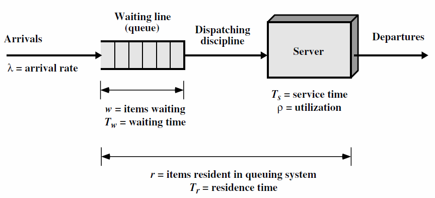 Figure 2.1 shows the arrival of the customer λ in erlang units, the system provides a maximum waiting room w with each customer having a waiting time of Tw, and there is a waiter s with service time Ts where the level of activity is p. Tr is the average time a customer waits in the system, and r is the number of customers in the system. For calculations, see the following image (Stalling, 1998): 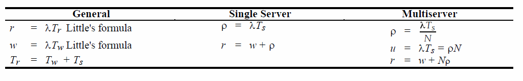 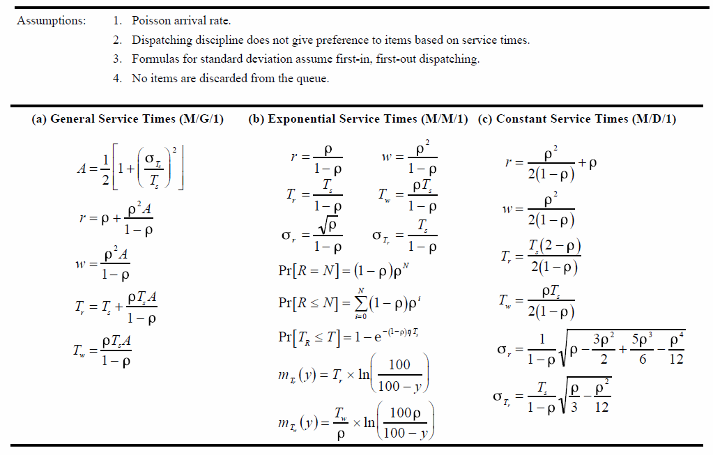 2.2 Droptail and RED (Random Early Detection) QueueDroptail uses a basic queue, namely FIFO (first in first out) by discarding packets when the buffer at the node is full, while Random Early Detection instructs a connection to slow down before the buffer is full. The aim of RED is congestion avoidance to avoid congestion rather than to overcome, global synchronization avoidance, avoidance of bias against bursty traffic, and bound on average queue length to maintain the average queue length so that it maintains the average delay. In general, the algorithm from RED is that the average queue length is less than the minimum limit, so the packet will be queued. If the average queue length is between the minimum and maximum limits, there will be a probability of discarding the package. If it is above the maximum, the package will be discarded (Stallings, 1998). 2.3 Network Simulator 3ns-3 is a discrete event network simulator, targeted primarily for research and educational use. ns-3 is free software, licensed under the GNU GPLv2 license, and the public for research, development and use (ns3-project, 2012). Chapter 3 Experimental Method3.1 Place and Time of ExperimentThe experiment was carried out at home on May 30, 2013. 3.2 Tools
3.3 ProgramThe first program takes an example from John Abraham, namely the comparison of Droptail with RED. The second program is about REDQueue by Marcos Talau and Duy Nguyen. /* -*- Mode:C++; c-file-style:"gnu"; indent-tabs-mode:nil; -*- */ /* * This program is free software; you can redistribute it and/or modify * it under the terms of the GNU General Public License version 2 as * published by the Free Software Foundation; * * This program is distributed in the hope that it will be useful, * but WITHOUT ANY WARRANTY; without even the implied warranty of * MERCHANTABILITY or FITNESS FOR A PARTICULAR PURPOSE. See the * GNU General Public License for more details. * * You should have received a copy of the GNU General Public License * along with this program; if not, write to the Free Software * Foundation, Inc., 59 Temple Place, Suite 330, Boston, MA 02111-1307 USA * * Author: John Abraham * */ #include "ns3/core-module.h" #include "ns3/network-module.h" #include "ns3/internet-module.h" #include "ns3/point-to-point-module.h" #include "ns3/applications-module.h" #include "ns3/point-to-point-layout-module.h" #include #include #include Code 3.1 Droptail_vs_RED.cc Program
/* -*- Mode:C++; c-file-style:"gnu"; indent-tabs-mode:nil; -*- */
/*
 * This program is free software; you can redistribute it and/or modify
 * it under the terms of the GNU General Public License version 2 as
 * published by the Free Software Foundation;
 *
 * This program is distributed in the hope that it will be useful,
 * but WITHOUT ANY WARRANTY; without even the implied warranty of
 * MERCHANTABILITY or FITNESS FOR A PARTICULAR PURPOSE. See the
 * GNU General Public License for more details.
 *
 * You should have received a copy of the GNU General Public License
 * along with this program; if not, write to the Free Software
 * Foundation, Inc., 59 Temple Place, Suite 330, Boston, MA 02111-1307 USA
 *
 * Authors: Marcos Talau
 * Duy Nguyen
 *
 */

#include "ns3/core-module.h"
#include "ns3/network-module.h"
#include "ns3/internet-module.h"
#include "ns3/flow-monitor-helper.h"
#include "ns3/point-to-point-module.h"
#include "ns3/applications-module.h"

using namespace ns3;

NS_LOG_COMPONENT_DEFINE ("RedTests");

uint32_t checkTimes;
double avgQueueSize;

// The times
double global_start_time;
double global_stop_time;
double sink_start_time;
double sink_stop_time;
double client_start_time;
double client_stop_time;

NodeContainer n0n2;
NodeContainer n1n2;
NodeContainer n2n3;
NodeContainer n3n4;
NodeContainer n3n5;

Ipv4InterfaceContainer i0i2;
Ipv4InterfaceContainer i1i2;
Ipv4InterfaceContainer i2i3;
Ipv4InterfaceContainer i3i4;
Ipv4InterfaceContainer i3i5;

std::stringstream filePlotQueue;
std::stringstream filePlotQueueAvg;

void
CheckQueueSize (Ptr queue)
{
 uint32_t qSize = StaticCast (queue)->GetQueueSize ();

 avgQueueSize += qSize;
 checkTimes++;

 // check queue size every 1/100 of a second
 Simulator::Schedule (Seconds (0.01), &CheckQueueSize, queue);

 std::ofstream fPlotQueue (filePlotQueue.str ().c_str (), std::ios::out|std::ios::app);
 fPlotQueue << Simulator::Now ().GetSeconds () << " " << qSize << std::endl;
 fPlotQueue.close ();

 std::ofstream fPlotQueueAvg (filePlotQueueAvg.str ().c_str (), std::ios::out|std::ios::app);
 fPlotQueueAvg << Simulator::Now ().GetSeconds () << " " << avgQueueSize / checkTimes << std::endl;
 fPlotQueueAvg.close ();
}

void
BuildAppsTest (uint32_t test)
{
 if ( (test == 1) || (test == 3) )
 {
 // SINK is in the right side
 uint16_t port = 50000;
 Address sinkLocalAddress (InetSocketAddress (Ipv4Address::GetAny (), port));
 PacketSinkHelper sinkHelper ("ns3::TcpSocketFactory", sinkLocalAddress);
 ApplicationContainer sinkApp = sinkHelper.Install (n3n4.Get (1));
 sinkApp.Start (Seconds (sink_start_time));
 sinkApp.Stop (Seconds (sink_stop_time));

 // Connection one
 // Clients are in left side
 /*
 * Create the OnOff applications to send TCP to the server
 * onoffhelper is a client that send data to TCP destination
 */
 OnOffHelper clientHelper1 ("ns3::TcpSocketFactory", Address ());
 clientHelper1.SetAttribute ("OnTime", StringValue ("ns3::ConstantRandomVariable[Constant=1]"));
 clientHelper1.SetAttribute ("OffTime", StringValue ("ns3::ConstantRandomVariable[Constant=0]"));
 clientHelper1.SetAttribute
 ("DataRate", DataRateValue (DataRate ("10Mb/s")));
 clientHelper1.SetAttribute
 ("PacketSize", UintegerValue (1000));

 ApplicationContainer clientApps1;
 AddressValue remoteAddress
 (InetSocketAddress (i3i4.GetAddress (1), port));
 clientHelper1.SetAttribute ("Remote", remoteAddress);
 clientApps1.Add (clientHelper1.Install (n0n2.Get (0)));
 clientApps1.Start (Seconds (client_start_time));
 clientApps1.Stop (Seconds (client_stop_time));

 // Connection two
 OnOffHelper clientHelper2 ("ns3::TcpSocketFactory", Address ());
 clientHelper2.SetAttribute ("OnTime", StringValue ("ns3::ConstantRandomVariable[Constant=1]"));
 clientHelper2.SetAttribute ("OffTime", StringValue ("ns3::ConstantRandomVariable[Constant=0]"));
 clientHelper2.SetAttribute
 ("DataRate", DataRateValue (DataRate ("10Mb/s")));
 clientHelper2.SetAttribute
 ("PacketSize", UintegerValue (1000));

 ApplicationContainer clientApps2;
 clientHelper2.SetAttribute ("Remote", remoteAddress);
 clientApps2.Add (clientHelper2.Install (n1n2.Get (0)));
 clientApps2.Start (Seconds (3.0));
 clientApps2.Stop (Seconds (client_stop_time));
 }
 else // 4 or 5
 {
 // SINKs
 // #1
 uint16_t port1 = 50001;
 Address sinkLocalAddress1 (InetSocketAddress (Ipv4Address::GetAny (), port1));
 PacketSinkHelper sinkHelper1 ("ns3::TcpSocketFactory", sinkLocalAddress1);
 ApplicationContainer sinkApp1 = sinkHelper1.Install (n3n4.Get (1));
 sinkApp1.Start (Seconds (sink_start_time));
 sinkApp1.Stop (Seconds (sink_stop_time));
 // #2
 uint16_t port2 = 50002;
 Address sinkLocalAddress2 (InetSocketAddress (Ipv4Address::GetAny (), port2));
 PacketSinkHelper sinkHelper2 ("ns3::TcpSocketFactory", sinkLocalAddress2);
 ApplicationContainer sinkApp2 = sinkHelper2.Install (n3n5.Get (1));
 sinkApp2.Start (Seconds (sink_start_time));
 sinkApp2.Stop (Seconds (sink_stop_time));
 // #3
 uint16_t port3 = 50003;
 Address sinkLocalAddress3 (InetSocketAddress (Ipv4Address::GetAny (), port3));
 PacketSinkHelper sinkHelper3 ("ns3::TcpSocketFactory", sinkLocalAddress3);
 ApplicationContainer sinkApp3 = sinkHelper3.Install (n0n2.Get (0));
 sinkApp3.Start (Seconds (sink_start_time));
 sinkApp3.Stop (Seconds (sink_stop_time));
 // #4
 uint16_t port4 = 50004;
 Address sinkLocalAddress4 (InetSocketAddress (Ipv4Address::GetAny (), port4));
 PacketSinkHelper sinkHelper4 ("ns3::TcpSocketFactory", sinkLocalAddress4);
 ApplicationContainer sinkApp4 = sinkHelper4.Install (n1n2.Get (0));
 sinkApp4.Start (Seconds (sink_start_time));
 sinkApp4.Stop (Seconds (sink_stop_time));

 // Connection #1
 /*
 * Create the OnOff applications to send TCP to the server
 * onoffhelper is a client that send data to TCP destination
 */
 OnOffHelper clientHelper1 ("ns3::TcpSocketFactory", Address ());
 clientHelper1.SetAttribute ("OnTime", StringValue ("ns3::ConstantRandomVariable[Constant=1]"));
 clientHelper1.SetAttribute ("OffTime", StringValue ("ns3::ConstantRandomVariable[Constant=0]"));
 clientHelper1.SetAttribute
 ("DataRate", DataRateValue (DataRate ("10Mb/s")));
 clientHelper1.SetAttribute
 ("PacketSize", UintegerValue (1000));

 ApplicationContainer clientApps1;
 AddressValue remoteAddress1
 (InetSocketAddress (i3i4.GetAddress (1), port1));
 clientHelper1.SetAttribute ("Remote", remoteAddress1);
 clientApps1.Add (clientHelper1.Install (n0n2.Get (0)));
 clientApps1.Start (Seconds (client_start_time));
 clientApps1.Stop (Seconds (client_stop_time));

 // Connection #2
 OnOffHelper clientHelper2 ("ns3::TcpSocketFactory", Address ());
 clientHelper2.SetAttribute ("OnTime", StringValue ("ns3::ConstantRandomVariable[Constant=1]"));
 clientHelper2.SetAttribute ("OffTime", StringValue ("ns3::ConstantRandomVariable[Constant=0]"));
 clientHelper2.SetAttribute
 ("DataRate", DataRateValue (DataRate ("10Mb/s")));
 clientHelper2.SetAttribute
 ("PacketSize", UintegerValue (1000));

 ApplicationContainer clientApps2;
 AddressValue remoteAddress2
 (InetSocketAddress (i3i5.GetAddress (1), port2));
 clientHelper2.SetAttribute ("Remote", remoteAddress2);
 clientApps2.Add (clientHelper2.Install (n1n2.Get (0)));
 clientApps2.Start (Seconds (2.0));
 clientApps2.Stop (Seconds (client_stop_time));

 // Connection #3
 OnOffHelper clientHelper3 ("ns3::TcpSocketFactory", Address ());
 clientHelper3.SetAttribute ("OnTime", StringValue ("ns3::ConstantRandomVariable[Constant=1]"));
 clientHelper3.SetAttribute ("OffTime", StringValue ("ns3::ConstantRandomVariable[Constant=0]"));
 clientHelper3.SetAttribute
 ("DataRate", DataRateValue (DataRate ("10Mb/s")));
 clientHelper3.SetAttribute
 ("PacketSize", UintegerValue (1000));

 ApplicationContainer clientApps3;
 AddressValue remoteAddress3
 (InetSocketAddress (i0i2.GetAddress (0), port3));
 clientHelper3.SetAttribute ("Remote", remoteAddress3);
 clientApps3.Add (clientHelper3.Install (n3n4.Get (1)));
 clientApps3.Start (Seconds (3.5));
 clientApps3.Stop (Seconds (client_stop_time));

 // Connection #4
 OnOffHelper clientHelper4 ("ns3::TcpSocketFactory", Address ());
 clientHelper4.SetAttribute ("OnTime", StringValue ("ns3::ConstantRandomVariable[Constant=1]"));
 clientHelper4.SetAttribute ("OffTime", StringValue ("ns3::ConstantRandomVariable[Constant=0]"));
 clientHelper4.SetAttribute
 ("DataRate", DataRateValue (DataRate ("40b/s")));
 clientHelper4.SetAttribute
 ("PacketSize", UintegerValue (5 * 8)); // telnet

 ApplicationContainer clientApps4;
 AddressValue remoteAddress4
 (InetSocketAddress (i1i2.GetAddress (0), port4));
 clientHelper4.SetAttribute ("Remote", remoteAddress4);
 clientApps4.Add (clientHelper4.Install (n3n5.Get (1)));
 clientApps4.Start (Seconds (1.0));
 clientApps4.Stop (Seconds (client_stop_time));
 }
}

int
main (int argc, char *argv[])
{
 // LogComponentEnable ("RedExamples", LOG_LEVEL_INFO);
 // LogComponentEnable ("TcpNewReno", LOG_LEVEL_INFO);
 // LogComponentEnable ("RedQueue", LOG_LEVEL_FUNCTION);
 LogComponentEnable ("RedQueue", LOG_LEVEL_INFO);

 uint32_t redTest;
 std::string redLinkDataRate = "1.5Mbps";
 std::string redLinkDelay = "20ms";

 std::string pathOut;
 bool writeForPlot = false;
 bool writePcap = false;
 bool flowMonitor = false;

 bool printRedStats = true;

 global_start_time = 0.0;
 global_stop_time = 11;
 sink_start_time = global_start_time;
 sink_stop_time = global_stop_time + 3.0;
 client_start_time = sink_start_time + 0.2;
 client_stop_time = global_stop_time - 2.0;

 // Configuration and command line parameter parsing
 redTest = 1;
 // Will only save in the directory if enable opts below
 pathOut = "."; // Current directory
 CommandLine cmd;
 cmd.AddValue ("testNumber", "Run test 1, 3, 4 or 5", redTest);
 cmd.AddValue ("pathOut", "Path to save results from --writeForPlot/--writePcap/--writeFlowMonitor", pathOut);
 cmd.AddValue ("writeForPlot", "<0/1> to write results for plot (gnuplot)", writeForPlot);
 cmd.AddValue ("writePcap", "<0/1> to write results in pcapfile", writePcap);
 cmd.AddValue ("writeFlowMonitor", "<0/1> to enable Flow Monitor and write their results", flowMonitor);

 cmd.Parse (argc, argv);
 if ( (redTest != 1) && (redTest != 3) && (redTest != 4) && (redTest != 5) )
 {
 NS_ABORT_MSG ("Invalid test number. Supported tests are 1, 3, 4 or 5");
 }

 NS_LOG_INFO ("Create nodes");
 NodeContainer c;
 c.Create (6);
 Names::Add ( "N0", c.Get (0));
 Names::Add ( "N1", c.Get (1));
 Names::Add ( "N2", c.Get (2));
 Names::Add ( "N3", c.Get (3));
 Names::Add ( "N4", c.Get (4));
 Names::Add ( "N5", c.Get (5));
 n0n2 = NodeContainer (c.Get (0), c.Get (2));
 n1n2 = NodeContainer (c.Get (1), c.Get (2));
 n2n3 = NodeContainer (c.Get (2), c.Get (3));
 n3n4 = NodeContainer (c.Get (3), c.Get (4));
 n3n5 = NodeContainer (c.Get (3), c.Get (5));

 Config::SetDefault ("ns3::TcpL4Protocol::SocketType", StringValue ("ns3::TcpReno"));
 // 42 = headers size
 Config::SetDefault ("ns3::TcpSocket::SegmentSize", UintegerValue (1000 - 42));
 Config::SetDefault ("ns3::TcpSocket::DelAckCount", UintegerValue (1));
 GlobalValue::Bind ("ChecksumEnabled", BooleanValue (false));

 uint32_t meanPktSize = 500;

 // RED params
 NS_LOG_INFO ("Set RED params");
 Config::SetDefault ("ns3::RedQueue::Mode", StringValue ("QUEUE_MODE_PACKETS"));
 Config::SetDefault ("ns3::RedQueue::MeanPktSize", UintegerValue (meanPktSize));
 Config::SetDefault ("ns3::RedQueue::Wait", BooleanValue (true));
 Config::SetDefault ("ns3::RedQueue::Gentle", BooleanValue (true));
 Config::SetDefault ("ns3::RedQueue::QW", DoubleValue (0.002));
 Config::SetDefault ("ns3::RedQueue::MinTh", DoubleValue (5));
 Config::SetDefault ("ns3::RedQueue::MaxTh", DoubleValue (15));
 Config::SetDefault ("ns3::RedQueue::QueueLimit", UintegerValue (25));

 if (redTest == 3) // test like 1, but with bad params
 {
 Config::SetDefault ("ns3::RedQueue::MaxTh", DoubleValue (10));
 Config::SetDefault ("ns3::RedQueue::QW", DoubleValue (0.003));
 }
 else if (redTest == 5) // test 5, same of test 4, but in byte mode
 {
 Config::SetDefault ("ns3::RedQueue::Mode", StringValue ("QUEUE_MODE_BYTES"));
 Config::SetDefault ("ns3::RedQueue::Ns1Compat", BooleanValue (true));
 Config::SetDefault ("ns3::RedQueue::MinTh", DoubleValue (5 * meanPktSize));
 Config::SetDefault ("ns3::RedQueue::MaxTh", DoubleValue (15 * meanPktSize));
 Config::SetDefault ("ns3::RedQueue::QueueLimit", UintegerValue (25 * meanPktSize));
 }

 NS_LOG_INFO ("Install internet stack on all nodes.");
 InternetStackHelper internet;
 internet.Install (c);

 NS_LOG_INFO ("Create channels");
 PointToPointHelper p2p;

 p2p.SetQueue ("ns3::DropTailQueue");
 p2p.SetDeviceAttribute ("DataRate", StringValue ("10Mbps"));
 p2p.SetChannelAttribute ("Delay", StringValue ("2ms"));
 NetDeviceContainer devn0n2 = p2p.Install (n0n2);

 p2p.SetQueue ("ns3::DropTailQueue");
 p2p.SetDeviceAttribute ("DataRate", StringValue ("10Mbps"));
 p2p.SetChannelAttribute ("Delay", StringValue ("3ms"));
 NetDeviceContainer devn1n2 = p2p.Install (n1n2);

 p2p.SetQueue ("ns3::RedQueue", // only backbone link has RED queue
 "LinkBandwidth", StringValue (redLinkDataRate),
 "LinkDelay", StringValue (redLinkDelay));
 p2p.SetDeviceAttribute ("DataRate", StringValue (redLinkDataRate));
 p2p.SetChannelAttribute ("Delay", StringValue (redLinkDelay));
 NetDeviceContainer devn2n3 = p2p.Install (n2n3);

 p2p.SetQueue ("ns3::DropTailQueue");
 p2p.SetDeviceAttribute ("DataRate", StringValue ("10Mbps"));
 p2p.SetChannelAttribute ("Delay", StringValue ("4ms"));
 NetDeviceContainer devn3n4 = p2p.Install (n3n4);

 p2p.SetQueue ("ns3::DropTailQueue");
 p2p.SetDeviceAttribute ("DataRate", StringValue ("10Mbps"));
 p2p.SetChannelAttribute ("Delay", StringValue ("5ms"));
 NetDeviceContainer devn3n5 = p2p.Install (n3n5);

 NS_LOG_INFO ("Assign IP Addresses");
 Ipv4AddressHelper ipv4;

 ipv4.SetBase ("10.1.1.0", "255.255.255.0");
 i0i2 = ipv4.Assign (devn0n2);

 ipv4.SetBase ("10.1.2.0", "255.255.255.0");
 i1i2 = ipv4.Assign (devn1n2);

 ipv4.SetBase ("10.1.3.0", "255.255.255.0");
 i2i3 = ipv4.Assign (devn2n3);

 ipv4.SetBase ("10.1.4.0", "255.255.255.0");
 i3i4 = ipv4.Assign (devn3n4);

 ipv4.SetBase ("10.1.5.0", "255.255.255.0");
 i3i5 = ipv4.Assign (devn3n5);

 // Set up the routing
 Ipv4GlobalRoutingHelper::PopulateRoutingTables ();

 if (redTest == 5)
 {
 // like in ns2 test, r2 -> r1, have a queue in packet mode
 Ptr nd = StaticCast (devn2n3.Get (1));
 Ptr queue = nd->GetQueue ();

 StaticCast (queue)->SetMode (RedQueue::QUEUE_MODE_PACKETS);
 StaticCast (queue)->SetTh (5, 15);
 StaticCast (queue)->SetQueueLimit (25);
 }

 BuildAppsTest (redTest);

 if (writePcap)
 {
 PointToPointHelper ptp;
 std::stringstream stmp;
 stmp << pathOut << "/red";
 ptp.EnablePcapAll (stmp.str ().c_str ());
 }

 Ptr flowmon;
 if (flowMonitor)
 {
 FlowMonitorHelper flowmonHelper;
 flowmon = flowmonHelper.InstallAll ();
 }

 if (writeForPlot)
 {
 filePlotQueue << pathOut << "/" << "red-queue.plotme";
 filePlotQueueAvg << pathOut << "/" << "red-queue_avg.plotme";

 remove (filePlotQueue.str ().c_str ());
 remove (filePlotQueueAvg.str ().c_str ());
 Ptr nd = StaticCast (devn2n3.Get (0));
 Ptr queue = nd->GetQueue ();
 Simulator::ScheduleNow (&CheckQueueSize, queue);
 }

 Simulator::Stop (Seconds (sink_stop_time));
 Simulator::Run ();

 if (flowMonitor)
 {
 std::stringstream stmp;
 stmp << pathOut << "/red.flowmon";

 flowmon->SerializeToXmlFile (stmp.str ().c_str (), false, false);
 }

 if (printRedStats)
 {
 Ptr nd = StaticCast (devn2n3.Get (0));
 RedQueue::Stats st = StaticCast (nd->GetQueue ())->GetStats ();
 std::cout << "*** RED stats from Node 2 queue ***" << std::endl;
 std::cout << "\t " << st.unforcedDrop << " drops due prob mark" << std::endl;
 std::cout << "\t " << st.forcedDrop << " drops due hard mark" << std::endl;
 std::cout << "\t " << st.qLimDrop << " drops due queue full" << std::endl;

 nd = StaticCast (devn2n3.Get (1));
 st = StaticCast (nd->GetQueue ())->GetStats ();
 std::cout << "*** RED stats from Node 3 queue ***" << std::endl;
 std::cout << "\t " << st.unforcedDrop << " drops due prob mark" << std::endl;
 std::cout << "\t " << st.forcedDrop << " drops due hard mark" << std::endl;
 std::cout << "\t " << st.qLimDrop << " drops due queue full" << std::endl;
 }

 Simulator::Destroy ();

 return 0;
}
Code 3.2 red_tests.cc Program Chapter 4 Discussion4.1 Droptail and RED comparison simulationIt can be seen in Figure 4.1 and Figure 4.2 that according to Stallings, 1998, the droptail node will wait until the queue capacity is full before dumping it, so that a large decrease in speed is seen, which is around 300 Kbps at full time. 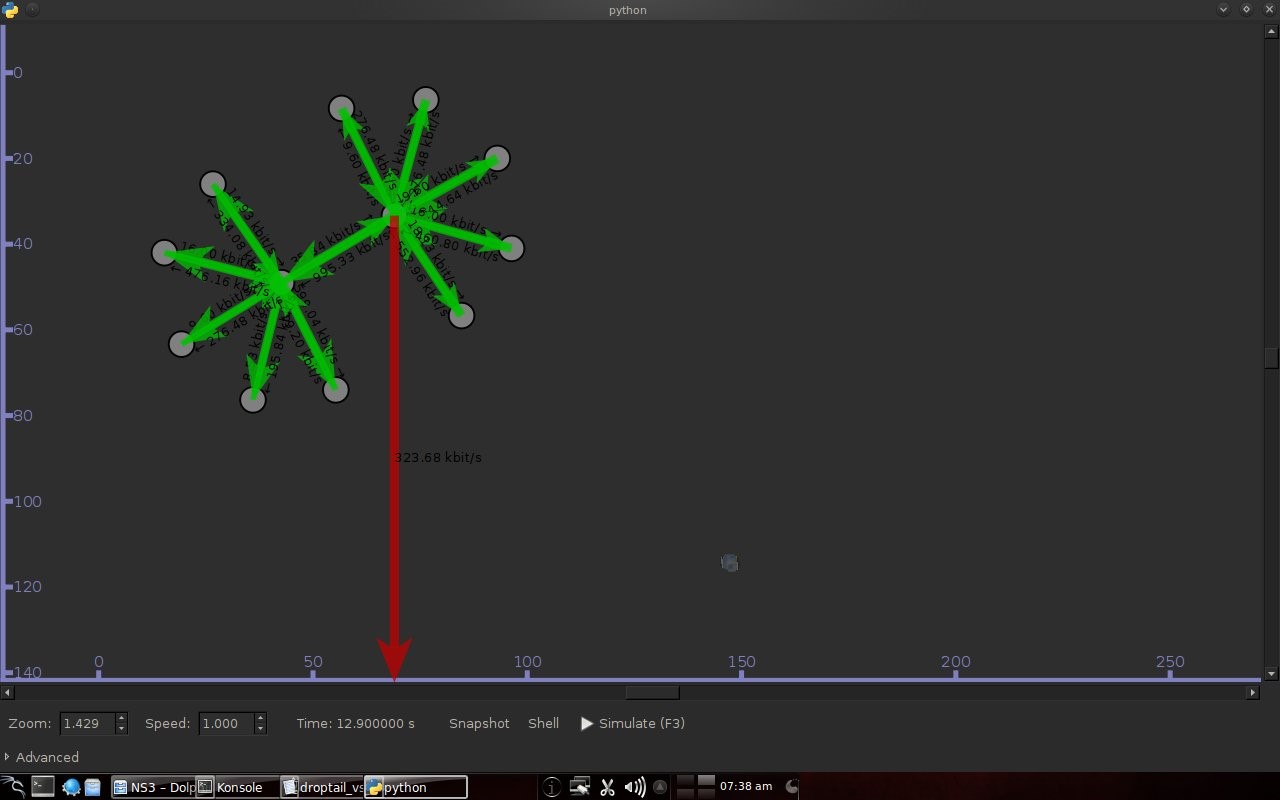 Meanwhile, in RED there is a preventive effort so that the capacity will not be full so disposal occurs before full capacity. Disposal of packages occurs based on the potential for excess capacity. So that you can see a gradual decrease in speed but not as big as in Droptail, which is around 50 Kbps. 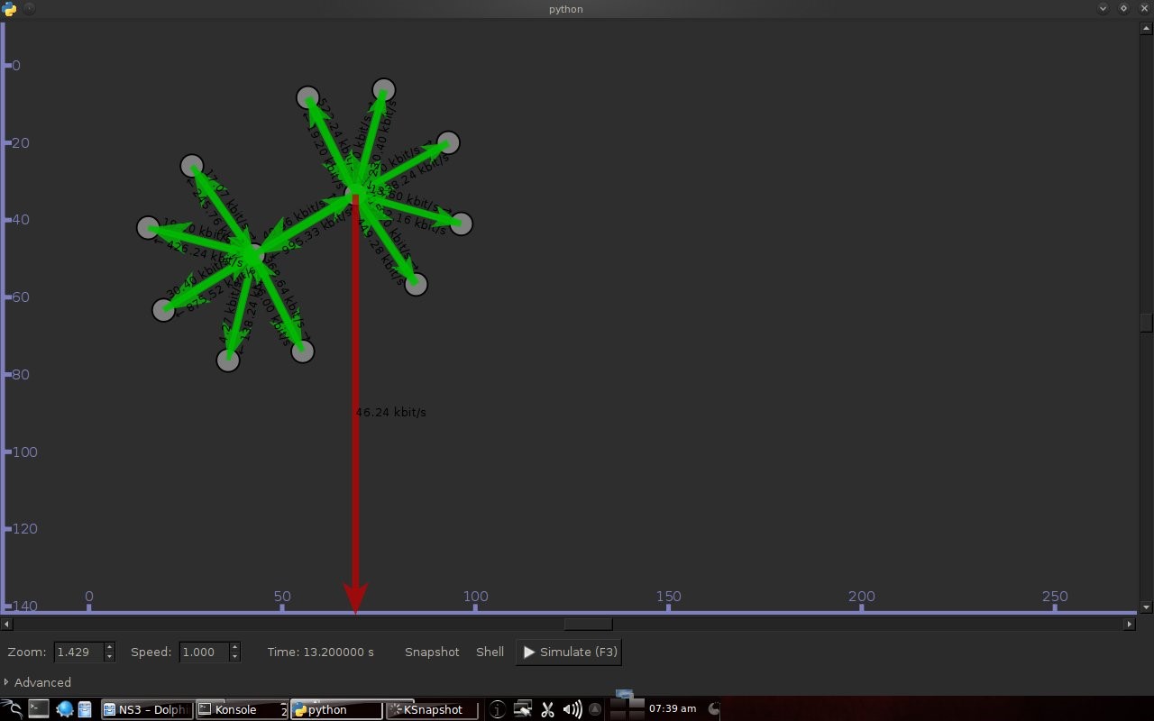 4.2 RED simulation on simple topologyFirst, initialization occurs, namely adjustment with a very large decrease in speed, which is around 1000 Kbps. 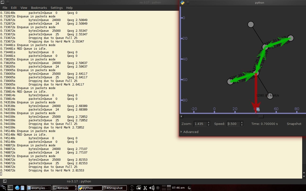 After that, it can be seen in Figure 4.4 that the node tries to keep the capacity from exceeding 25,000 packages by gradually decreasing the speed. In the figure after Figure 4.4 the node decreases speed gradually in terms of the potential for full capacity. According to Stallings, 1998, REDQueue's work is that packets will queue if the average queue capacity does not exceed the minimum limit specified by RED. If the average queue capacity is between the minimum and the maximum limits then disposal occurs based on the probability that full capacity will occur. If the average queue capacity exceeds the maximum limit, a package discard will occur. It can be seen in the next result according to the theory. 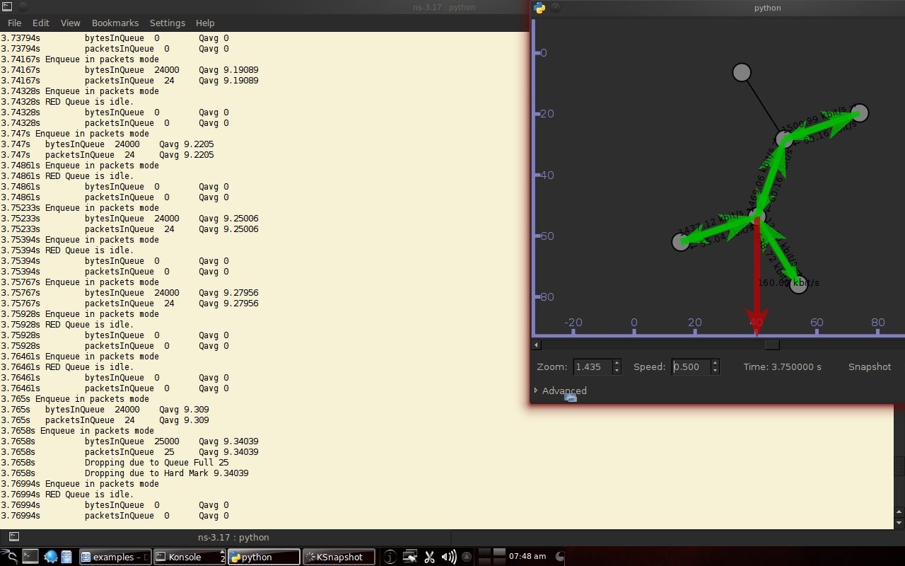 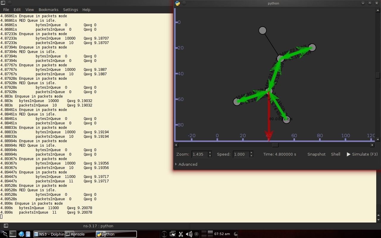 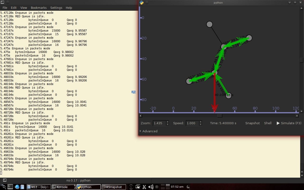 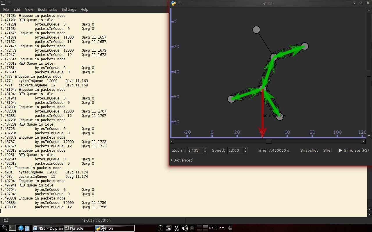 Chapter 5 Closing5.1 ConclusionNetwork Simulator 3 can simulate REDQueue and display animation so it's easier to observe. While this simple queue simulation is in accordance with the theory where the animation shows packet dumping in the droptail when the traffic exceeds the capacity which could potentially be negative on the system, whereas in random early detection (RED) the animation shows packet dumping before the traffic exceeds capacity which can reduce the negative potential on the system. 5.2 Future WorkThis simulation is just a simple experiment. Actually Network Simulator is made to simulate more complicated experiments. Bibliography
CatatanTulisan ini merupakan tugas S1 mata kuliah Sistem Antrean Telekomunikasi saya di Jurusan Teknik Elektro, Fakultas Teknik, Universitas Udayana. Tugas ini tidak pernah dipublikasi dimanapun dan saya sebagai penulis dan pemegang hak cipta melisensi tulisan ini customized CC-BY-SA dimana siapa saja boleh membagi, menyalin, mempublikasi ulang, dan menjualnya dengan syarat mencatumkan nama saya sebagai penulis dan memberitahu bahwa versi asli dan terbuka ada disini. BAB 1 Pendahuluan1.1 Latar BelakangTeori antrean merupakan suatu teori dimana pelanggan harus antri untuk mendapatkan pelayanan dari pelayan. Teori antrean bertujuan untuk mengatur tingkat pelayanan dengan data kedatangan pelanggan. Pada teori antrean terdapat cara untuk mengatur tingkat pelayanan yang tepat, tingkat kesibukkan pelayan, berapa lama suatu pelanggan harus menunggu, berapa jumlah pelanggan dalam antrean, berapa besar ruang tunggu yang harus disiapkan, dan lain-lain. Di dunia nyata suatu pelayanan tidak terlepas dari antrean, termasuk pelayanan pada jaringan data. Untuk mensimulasikan antrean pada jaringan data telah tersedia banyak perangkat lunak seperti Network Simulator, yang kini telah berkembang menjadi NS3 (Network Simulator 3). Pada NS3 antrean dapat diatur secara manual namun telah tersedia 2 jenis antrean yang sudah jadi yaitu Droptail dan RED(Random Early Detection)Queue. Sudah tersedia contoh yang dibuat oleh Marcos Talau dan Duy Nguyen. Pada makalah ini akan disimulasikan REDQueue pada jaringan komputer point-to-point sederhana. 1.2 Rumusan MasalahBagaimana simulasi REDQueue yang telah disediakan oleh Marcos Talau dan Duy Nguyen? 1.3 TujuanUntuk mensimulasikan REDQueue oleh Marcos Talau dan Duy Nguyen pada NS3. 1.4 Manfaat
1.5 Ruang Lingkup dan Batasan
BAB 2 Tinjauan Pustaka2.1 AntreanModel antrean sederhana dapat dilihat seperti berikut: Pada gambar 2.1 terlihat kedatangan pelanggan λ dalam satuan erlang, pada sistem disediakan ruang tunggu maksimum w dengan masing-masing pelanggan ada waktu tunggu Tw, dan ada pelayan s dengan waktu pelayanan Ts dimana tingkat kesibukannya adalah p. Tr merupakan waktu rata – rata suatu pelanggan menunggu di sistem, dan r merupakan jumlah pelanggan dalam sistem. Untuk perhitungan dapat dilihat gambar berikut (Stalling, 1998): 2.2 Droptail dan RED (Random Early Detection) QueueDroptail menggunakan antrean dasar yaitu FIFO (first in first out) dengan membuang paket bila buffer pada node penuh, sedangkan Random Early Detection memerintahkan suatu koneksi untuk mengurangi kecepatan sebelum buffer penuh. Tujuan RED adalah congestion avoidance lebih untuk menghindari kongesti dari pada mengatasi, global synchronization avoidance, Avoidance of bias against bursty traffic, dan bound on average queue length untuk mempertahankan rata-rata panjang antrean maka mempertahankan rata-rata delay. Secara umum algoritma dari RED adalah rata-rata panjang antrean lebih kecil dari batasan minimal yang ditentukan, maka paket akan antre. Bila rata-rata panjang antrean diantara batasan minimal dan batasan maksimal maka akan ada probabiltas pembuangan paket. Bila diatas maksimal maka akan terjadi pembuangan paket (Stallings, 1998). 2.3 Network Simulator 3ns-3 adalah simulator jaringan kejadian diskrit, ditargetkan terutama untuk penelitian dan penggunaan pendidikan. ns-3 adalah perangkat lunak bebas, dilisensikan di bawah lisensi GNU GPLv2, dan publik untuk penelitian, pengembangan, dan penggunaan (ns3-project, 2012). BAB 3 Metode Percobaan3.1 Tempat dan Waktu PercobaanPercobaan dilakukan di Rumah pada tanggal 30 Mei 2013. 3.2 Alat
3.3 ProgramProgram pertama mengambil contoh dari John Abraham yaitu perbandingan Droptail dengan RED. Program kedua adalah tentang REDQueue dari Marcos Talau dan Duy Nguyen. /* -*- Mode:C++; c-file-style:"gnu"; indent-tabs-mode:nil; -*- */ /* * This program is free software; you can redistribute it and/or modify * it under the terms of the GNU General Public License version 2 as * published by the Free Software Foundation; * * This program is distributed in the hope that it will be useful, * but WITHOUT ANY WARRANTY; without even the implied warranty of * MERCHANTABILITY or FITNESS FOR A PARTICULAR PURPOSE. See the * GNU General Public License for more details. * * You should have received a copy of the GNU General Public License * along with this program; if not, write to the Free Software * Foundation, Inc., 59 Temple Place, Suite 330, Boston, MA 02111-1307 USA * * Author: John Abraham * */ #include "ns3/core-module.h" #include "ns3/network-module.h" #include "ns3/internet-module.h" #include "ns3/point-to-point-module.h" #include "ns3/applications-module.h" #include "ns3/point-to-point-layout-module.h" #include #include #include Kode 3.1 Program Droptail_vs_RED.cc
/* -*- Mode:C++; c-file-style:"gnu"; indent-tabs-mode:nil; -*- */
/*
 * This program is free software; you can redistribute it and/or modify
 * it under the terms of the GNU General Public License version 2 as
 * published by the Free Software Foundation;
 *
 * This program is distributed in the hope that it will be useful,
 * but WITHOUT ANY WARRANTY; without even the implied warranty of
 * MERCHANTABILITY or FITNESS FOR A PARTICULAR PURPOSE. See the
 * GNU General Public License for more details.
 *
 * You should have received a copy of the GNU General Public License
 * along with this program; if not, write to the Free Software
 * Foundation, Inc., 59 Temple Place, Suite 330, Boston, MA 02111-1307 USA
 *
 * Authors: Marcos Talau
 * Duy Nguyen
 *
 */

#include "ns3/core-module.h"
#include "ns3/network-module.h"
#include "ns3/internet-module.h"
#include "ns3/flow-monitor-helper.h"
#include "ns3/point-to-point-module.h"
#include "ns3/applications-module.h"

using namespace ns3;

NS_LOG_COMPONENT_DEFINE ("RedTests");

uint32_t checkTimes;
double avgQueueSize;

// The times
double global_start_time;
double global_stop_time;
double sink_start_time;
double sink_stop_time;
double client_start_time;
double client_stop_time;

NodeContainer n0n2;
NodeContainer n1n2;
NodeContainer n2n3;
NodeContainer n3n4;
NodeContainer n3n5;

Ipv4InterfaceContainer i0i2;
Ipv4InterfaceContainer i1i2;
Ipv4InterfaceContainer i2i3;
Ipv4InterfaceContainer i3i4;
Ipv4InterfaceContainer i3i5;

std::stringstream filePlotQueue;
std::stringstream filePlotQueueAvg;

void
CheckQueueSize (Ptr queue)
{
 uint32_t qSize = StaticCast (queue)->GetQueueSize ();

 avgQueueSize += qSize;
 checkTimes++;

 // check queue size every 1/100 of a second
 Simulator::Schedule (Seconds (0.01), &CheckQueueSize, queue);

 std::ofstream fPlotQueue (filePlotQueue.str ().c_str (), std::ios::out|std::ios::app);
 fPlotQueue << Simulator::Now ().GetSeconds () << " " << qSize << std::endl;
 fPlotQueue.close ();

 std::ofstream fPlotQueueAvg (filePlotQueueAvg.str ().c_str (), std::ios::out|std::ios::app);
 fPlotQueueAvg << Simulator::Now ().GetSeconds () << " " << avgQueueSize / checkTimes << std::endl;
 fPlotQueueAvg.close ();
}

void
BuildAppsTest (uint32_t test)
{
 if ( (test == 1) || (test == 3) )
 {
 // SINK is in the right side
 uint16_t port = 50000;
 Address sinkLocalAddress (InetSocketAddress (Ipv4Address::GetAny (), port));
 PacketSinkHelper sinkHelper ("ns3::TcpSocketFactory", sinkLocalAddress);
 ApplicationContainer sinkApp = sinkHelper.Install (n3n4.Get (1));
 sinkApp.Start (Seconds (sink_start_time));
 sinkApp.Stop (Seconds (sink_stop_time));

 // Connection one
 // Clients are in left side
 /*
 * Create the OnOff applications to send TCP to the server
 * onoffhelper is a client that send data to TCP destination
 */
 OnOffHelper clientHelper1 ("ns3::TcpSocketFactory", Address ());
 clientHelper1.SetAttribute ("OnTime", StringValue ("ns3::ConstantRandomVariable[Constant=1]"));
 clientHelper1.SetAttribute ("OffTime", StringValue ("ns3::ConstantRandomVariable[Constant=0]"));
 clientHelper1.SetAttribute
 ("DataRate", DataRateValue (DataRate ("10Mb/s")));
 clientHelper1.SetAttribute
 ("PacketSize", UintegerValue (1000));

 ApplicationContainer clientApps1;
 AddressValue remoteAddress
 (InetSocketAddress (i3i4.GetAddress (1), port));
 clientHelper1.SetAttribute ("Remote", remoteAddress);
 clientApps1.Add (clientHelper1.Install (n0n2.Get (0)));
 clientApps1.Start (Seconds (client_start_time));
 clientApps1.Stop (Seconds (client_stop_time));

 // Connection two
 OnOffHelper clientHelper2 ("ns3::TcpSocketFactory", Address ());
 clientHelper2.SetAttribute ("OnTime", StringValue ("ns3::ConstantRandomVariable[Constant=1]"));
 clientHelper2.SetAttribute ("OffTime", StringValue ("ns3::ConstantRandomVariable[Constant=0]"));
 clientHelper2.SetAttribute
 ("DataRate", DataRateValue (DataRate ("10Mb/s")));
 clientHelper2.SetAttribute
 ("PacketSize", UintegerValue (1000));

 ApplicationContainer clientApps2;
 clientHelper2.SetAttribute ("Remote", remoteAddress);
 clientApps2.Add (clientHelper2.Install (n1n2.Get (0)));
 clientApps2.Start (Seconds (3.0));
 clientApps2.Stop (Seconds (client_stop_time));
 }
 else // 4 or 5
 {
 // SINKs
 // #1
 uint16_t port1 = 50001;
 Address sinkLocalAddress1 (InetSocketAddress (Ipv4Address::GetAny (), port1));
 PacketSinkHelper sinkHelper1 ("ns3::TcpSocketFactory", sinkLocalAddress1);
 ApplicationContainer sinkApp1 = sinkHelper1.Install (n3n4.Get (1));
 sinkApp1.Start (Seconds (sink_start_time));
 sinkApp1.Stop (Seconds (sink_stop_time));
 // #2
 uint16_t port2 = 50002;
 Address sinkLocalAddress2 (InetSocketAddress (Ipv4Address::GetAny (), port2));
 PacketSinkHelper sinkHelper2 ("ns3::TcpSocketFactory", sinkLocalAddress2);
 ApplicationContainer sinkApp2 = sinkHelper2.Install (n3n5.Get (1));
 sinkApp2.Start (Seconds (sink_start_time));
 sinkApp2.Stop (Seconds (sink_stop_time));
 // #3
 uint16_t port3 = 50003;
 Address sinkLocalAddress3 (InetSocketAddress (Ipv4Address::GetAny (), port3));
 PacketSinkHelper sinkHelper3 ("ns3::TcpSocketFactory", sinkLocalAddress3);
 ApplicationContainer sinkApp3 = sinkHelper3.Install (n0n2.Get (0));
 sinkApp3.Start (Seconds (sink_start_time));
 sinkApp3.Stop (Seconds (sink_stop_time));
 // #4
 uint16_t port4 = 50004;
 Address sinkLocalAddress4 (InetSocketAddress (Ipv4Address::GetAny (), port4));
 PacketSinkHelper sinkHelper4 ("ns3::TcpSocketFactory", sinkLocalAddress4);
 ApplicationContainer sinkApp4 = sinkHelper4.Install (n1n2.Get (0));
 sinkApp4.Start (Seconds (sink_start_time));
 sinkApp4.Stop (Seconds (sink_stop_time));

 // Connection #1
 /*
 * Create the OnOff applications to send TCP to the server
 * onoffhelper is a client that send data to TCP destination
 */
 OnOffHelper clientHelper1 ("ns3::TcpSocketFactory", Address ());
 clientHelper1.SetAttribute ("OnTime", StringValue ("ns3::ConstantRandomVariable[Constant=1]"));
 clientHelper1.SetAttribute ("OffTime", StringValue ("ns3::ConstantRandomVariable[Constant=0]"));
 clientHelper1.SetAttribute
 ("DataRate", DataRateValue (DataRate ("10Mb/s")));
 clientHelper1.SetAttribute
 ("PacketSize", UintegerValue (1000));

 ApplicationContainer clientApps1;
 AddressValue remoteAddress1
 (InetSocketAddress (i3i4.GetAddress (1), port1));
 clientHelper1.SetAttribute ("Remote", remoteAddress1);
 clientApps1.Add (clientHelper1.Install (n0n2.Get (0)));
 clientApps1.Start (Seconds (client_start_time));
 clientApps1.Stop (Seconds (client_stop_time));

 // Connection #2
 OnOffHelper clientHelper2 ("ns3::TcpSocketFactory", Address ());
 clientHelper2.SetAttribute ("OnTime", StringValue ("ns3::ConstantRandomVariable[Constant=1]"));
 clientHelper2.SetAttribute ("OffTime", StringValue ("ns3::ConstantRandomVariable[Constant=0]"));
 clientHelper2.SetAttribute
 ("DataRate", DataRateValue (DataRate ("10Mb/s")));
 clientHelper2.SetAttribute
 ("PacketSize", UintegerValue (1000));

 ApplicationContainer clientApps2;
 AddressValue remoteAddress2
 (InetSocketAddress (i3i5.GetAddress (1), port2));
 clientHelper2.SetAttribute ("Remote", remoteAddress2);
 clientApps2.Add (clientHelper2.Install (n1n2.Get (0)));
 clientApps2.Start (Seconds (2.0));
 clientApps2.Stop (Seconds (client_stop_time));

 // Connection #3
 OnOffHelper clientHelper3 ("ns3::TcpSocketFactory", Address ());
 clientHelper3.SetAttribute ("OnTime", StringValue ("ns3::ConstantRandomVariable[Constant=1]"));
 clientHelper3.SetAttribute ("OffTime", StringValue ("ns3::ConstantRandomVariable[Constant=0]"));
 clientHelper3.SetAttribute
 ("DataRate", DataRateValue (DataRate ("10Mb/s")));
 clientHelper3.SetAttribute
 ("PacketSize", UintegerValue (1000));

 ApplicationContainer clientApps3;
 AddressValue remoteAddress3
 (InetSocketAddress (i0i2.GetAddress (0), port3));
 clientHelper3.SetAttribute ("Remote", remoteAddress3);
 clientApps3.Add (clientHelper3.Install (n3n4.Get (1)));
 clientApps3.Start (Seconds (3.5));
 clientApps3.Stop (Seconds (client_stop_time));

 // Connection #4
 OnOffHelper clientHelper4 ("ns3::TcpSocketFactory", Address ());
 clientHelper4.SetAttribute ("OnTime", StringValue ("ns3::ConstantRandomVariable[Constant=1]"));
 clientHelper4.SetAttribute ("OffTime", StringValue ("ns3::ConstantRandomVariable[Constant=0]"));
 clientHelper4.SetAttribute
 ("DataRate", DataRateValue (DataRate ("40b/s")));
 clientHelper4.SetAttribute
 ("PacketSize", UintegerValue (5 * 8)); // telnet

 ApplicationContainer clientApps4;
 AddressValue remoteAddress4
 (InetSocketAddress (i1i2.GetAddress (0), port4));
 clientHelper4.SetAttribute ("Remote", remoteAddress4);
 clientApps4.Add (clientHelper4.Install (n3n5.Get (1)));
 clientApps4.Start (Seconds (1.0));
 clientApps4.Stop (Seconds (client_stop_time));
 }
}

int
main (int argc, char *argv[])
{
 // LogComponentEnable ("RedExamples", LOG_LEVEL_INFO);
 // LogComponentEnable ("TcpNewReno", LOG_LEVEL_INFO);
 // LogComponentEnable ("RedQueue", LOG_LEVEL_FUNCTION);
 LogComponentEnable ("RedQueue", LOG_LEVEL_INFO);

 uint32_t redTest;
 std::string redLinkDataRate = "1.5Mbps";
 std::string redLinkDelay = "20ms";

 std::string pathOut;
 bool writeForPlot = false;
 bool writePcap = false;
 bool flowMonitor = false;

 bool printRedStats = true;

 global_start_time = 0.0;
 global_stop_time = 11;
 sink_start_time = global_start_time;
 sink_stop_time = global_stop_time + 3.0;
 client_start_time = sink_start_time + 0.2;
 client_stop_time = global_stop_time - 2.0;

 // Configuration and command line parameter parsing
 redTest = 1;
 // Will only save in the directory if enable opts below
 pathOut = "."; // Current directory
 CommandLine cmd;
 cmd.AddValue ("testNumber", "Run test 1, 3, 4 or 5", redTest);
 cmd.AddValue ("pathOut", "Path to save results from --writeForPlot/--writePcap/--writeFlowMonitor", pathOut);
 cmd.AddValue ("writeForPlot", "<0/1> to write results for plot (gnuplot)", writeForPlot);
 cmd.AddValue ("writePcap", "<0/1> to write results in pcapfile", writePcap);
 cmd.AddValue ("writeFlowMonitor", "<0/1> to enable Flow Monitor and write their results", flowMonitor);

 cmd.Parse (argc, argv);
 if ( (redTest != 1) && (redTest != 3) && (redTest != 4) && (redTest != 5) )
 {
 NS_ABORT_MSG ("Invalid test number. Supported tests are 1, 3, 4 or 5");
 }

 NS_LOG_INFO ("Create nodes");
 NodeContainer c;
 c.Create (6);
 Names::Add ( "N0", c.Get (0));
 Names::Add ( "N1", c.Get (1));
 Names::Add ( "N2", c.Get (2));
 Names::Add ( "N3", c.Get (3));
 Names::Add ( "N4", c.Get (4));
 Names::Add ( "N5", c.Get (5));
 n0n2 = NodeContainer (c.Get (0), c.Get (2));
 n1n2 = NodeContainer (c.Get (1), c.Get (2));
 n2n3 = NodeContainer (c.Get (2), c.Get (3));
 n3n4 = NodeContainer (c.Get (3), c.Get (4));
 n3n5 = NodeContainer (c.Get (3), c.Get (5));

 Config::SetDefault ("ns3::TcpL4Protocol::SocketType", StringValue ("ns3::TcpReno"));
 // 42 = headers size
 Config::SetDefault ("ns3::TcpSocket::SegmentSize", UintegerValue (1000 - 42));
 Config::SetDefault ("ns3::TcpSocket::DelAckCount", UintegerValue (1));
 GlobalValue::Bind ("ChecksumEnabled", BooleanValue (false));

 uint32_t meanPktSize = 500;

 // RED params
 NS_LOG_INFO ("Set RED params");
 Config::SetDefault ("ns3::RedQueue::Mode", StringValue ("QUEUE_MODE_PACKETS"));
 Config::SetDefault ("ns3::RedQueue::MeanPktSize", UintegerValue (meanPktSize));
 Config::SetDefault ("ns3::RedQueue::Wait", BooleanValue (true));
 Config::SetDefault ("ns3::RedQueue::Gentle", BooleanValue (true));
 Config::SetDefault ("ns3::RedQueue::QW", DoubleValue (0.002));
 Config::SetDefault ("ns3::RedQueue::MinTh", DoubleValue (5));
 Config::SetDefault ("ns3::RedQueue::MaxTh", DoubleValue (15));
 Config::SetDefault ("ns3::RedQueue::QueueLimit", UintegerValue (25));

 if (redTest == 3) // test like 1, but with bad params
 {
 Config::SetDefault ("ns3::RedQueue::MaxTh", DoubleValue (10));
 Config::SetDefault ("ns3::RedQueue::QW", DoubleValue (0.003));
 }
 else if (redTest == 5) // test 5, same of test 4, but in byte mode
 {
 Config::SetDefault ("ns3::RedQueue::Mode", StringValue ("QUEUE_MODE_BYTES"));
 Config::SetDefault ("ns3::RedQueue::Ns1Compat", BooleanValue (true));
 Config::SetDefault ("ns3::RedQueue::MinTh", DoubleValue (5 * meanPktSize));
 Config::SetDefault ("ns3::RedQueue::MaxTh", DoubleValue (15 * meanPktSize));
 Config::SetDefault ("ns3::RedQueue::QueueLimit", UintegerValue (25 * meanPktSize));
 }

 NS_LOG_INFO ("Install internet stack on all nodes.");
 InternetStackHelper internet;
 internet.Install (c);

 NS_LOG_INFO ("Create channels");
 PointToPointHelper p2p;

 p2p.SetQueue ("ns3::DropTailQueue");
 p2p.SetDeviceAttribute ("DataRate", StringValue ("10Mbps"));
 p2p.SetChannelAttribute ("Delay", StringValue ("2ms"));
 NetDeviceContainer devn0n2 = p2p.Install (n0n2);

 p2p.SetQueue ("ns3::DropTailQueue");
 p2p.SetDeviceAttribute ("DataRate", StringValue ("10Mbps"));
 p2p.SetChannelAttribute ("Delay", StringValue ("3ms"));
 NetDeviceContainer devn1n2 = p2p.Install (n1n2);

 p2p.SetQueue ("ns3::RedQueue", // only backbone link has RED queue
 "LinkBandwidth", StringValue (redLinkDataRate),
 "LinkDelay", StringValue (redLinkDelay));
 p2p.SetDeviceAttribute ("DataRate", StringValue (redLinkDataRate));
 p2p.SetChannelAttribute ("Delay", StringValue (redLinkDelay));
 NetDeviceContainer devn2n3 = p2p.Install (n2n3);

 p2p.SetQueue ("ns3::DropTailQueue");
 p2p.SetDeviceAttribute ("DataRate", StringValue ("10Mbps"));
 p2p.SetChannelAttribute ("Delay", StringValue ("4ms"));
 NetDeviceContainer devn3n4 = p2p.Install (n3n4);

 p2p.SetQueue ("ns3::DropTailQueue");
 p2p.SetDeviceAttribute ("DataRate", StringValue ("10Mbps"));
 p2p.SetChannelAttribute ("Delay", StringValue ("5ms"));
 NetDeviceContainer devn3n5 = p2p.Install (n3n5);

 NS_LOG_INFO ("Assign IP Addresses");
 Ipv4AddressHelper ipv4;

 ipv4.SetBase ("10.1.1.0", "255.255.255.0");
 i0i2 = ipv4.Assign (devn0n2);

 ipv4.SetBase ("10.1.2.0", "255.255.255.0");
 i1i2 = ipv4.Assign (devn1n2);

 ipv4.SetBase ("10.1.3.0", "255.255.255.0");
 i2i3 = ipv4.Assign (devn2n3);

 ipv4.SetBase ("10.1.4.0", "255.255.255.0");
 i3i4 = ipv4.Assign (devn3n4);

 ipv4.SetBase ("10.1.5.0", "255.255.255.0");
 i3i5 = ipv4.Assign (devn3n5);

 // Set up the routing
 Ipv4GlobalRoutingHelper::PopulateRoutingTables ();

 if (redTest == 5)
 {
 // like in ns2 test, r2 -> r1, have a queue in packet mode
 Ptr nd = StaticCast (devn2n3.Get (1));
 Ptr queue = nd->GetQueue ();

 StaticCast (queue)->SetMode (RedQueue::QUEUE_MODE_PACKETS);
 StaticCast (queue)->SetTh (5, 15);
 StaticCast (queue)->SetQueueLimit (25);
 }

 BuildAppsTest (redTest);

 if (writePcap)
 {
 PointToPointHelper ptp;
 std::stringstream stmp;
 stmp << pathOut << "/red";
 ptp.EnablePcapAll (stmp.str ().c_str ());
 }

 Ptr flowmon;
 if (flowMonitor)
 {
 FlowMonitorHelper flowmonHelper;
 flowmon = flowmonHelper.InstallAll ();
 }

 if (writeForPlot)
 {
 filePlotQueue << pathOut << "/" << "red-queue.plotme";
 filePlotQueueAvg << pathOut << "/" << "red-queue_avg.plotme";

 remove (filePlotQueue.str ().c_str ());
 remove (filePlotQueueAvg.str ().c_str ());
 Ptr nd = StaticCast (devn2n3.Get (0));
 Ptr queue = nd->GetQueue ();
 Simulator::ScheduleNow (&CheckQueueSize, queue);
 }

 Simulator::Stop (Seconds (sink_stop_time));
 Simulator::Run ();

 if (flowMonitor)
 {
 std::stringstream stmp;
 stmp << pathOut << "/red.flowmon";

 flowmon->SerializeToXmlFile (stmp.str ().c_str (), false, false);
 }

 if (printRedStats)
 {
 Ptr nd = StaticCast (devn2n3.Get (0));
 RedQueue::Stats st = StaticCast (nd->GetQueue ())->GetStats ();
 std::cout << "*** RED stats from Node 2 queue ***" << std::endl;
 std::cout << "\t " << st.unforcedDrop << " drops due prob mark" << std::endl;
 std::cout << "\t " << st.forcedDrop << " drops due hard mark" << std::endl;
 std::cout << "\t " << st.qLimDrop << " drops due queue full" << std::endl;

 nd = StaticCast (devn2n3.Get (1));
 st = StaticCast (nd->GetQueue ())->GetStats ();
 std::cout << "*** RED stats from Node 3 queue ***" << std::endl;
 std::cout << "\t " << st.unforcedDrop << " drops due prob mark" << std::endl;
 std::cout << "\t " << st.forcedDrop << " drops due hard mark" << std::endl;
 std::cout << "\t " << st.qLimDrop << " drops due queue full" << std::endl;
 }

 Simulator::Destroy ();

 return 0;
}
Kode 3.2 Program red_tests.cc BAB 4 Pembahasan4.1 Simulasi perbandingan Droptail dan REDTerlihat pada gambar 4.1 dan gambar 4.2 bekerja menurut Stallings, 1998, yaitu pada droptail simpul akan menunggu sampai kapasitas antrean penuh baru melakukan pembuangan, sehingga terlihat terjadi penurunan kecepatan yang besar yaitu sekitar 300 Kbps pada saat penuh. Sedangkan pada RED terjadi usaha pencegahan agar kapasitas tidak penuh sehingga telah terjadi pembuangan sebelum kapasitas penuh. Pembuangan paket terjadi berdasarkan potensi terjadinya kelebihan kapasitas. Sehingga terlihat penurun kecepatan bertahap tetapi tidak sebesar pada Droptail yaitu sekitar 50 Kbps. 4.2 Simulasi RED pada topologi sederhanaPertama terjadi inisialisasi yaitu penyesuaian dengan penurunnan kecepat yang sangat besar yaitu sekitar 1000 Kbps. Setelah itu terlihat pada gambar 4.4 simpul berusaha agar kapasitas tidak melebihi 25000 paket dengan melakukan penurunan speed secara bertahap. Pada gambar setelah gambar 4.4 simpul melakukan penurunan speed secara bertahap ditinjau dari potensi terjadi kapasitas penuh. Menurut Stallings, 1998, kerja REDQueue adalah paket akan antre bila kapasitas antrean rata-rata tidak melebihi batasan minimal yang ditentukan oleh RED. Bila kapasitas antrean rata-rata diatara batas minimal dan batas maksimal maka pembuangan terjadi berdasarkan probabilatas akan terjadinya kapasitas penuh. Bila kapasitas antrean rata-rata melembih batas maksimal maka akan terjadi pembuangan paket. Terlihat pada hasil berikutnya sesuai dengan teori. BAB 5 Penutup5.1 SimpulanNetwork Simulator 3 dapat mensimulasikan REDQueue dan menampilkan animasi sehingga lebih mudah untuk diamati. Sementara simulasi antrean yang sederhana ini sesuai dengan teori dimana animasi menunjukkan pembuangan paket pada droptail saat trafik melebihi kapasitas dan pada random early detection (RED) animasi menunjukkan pembuatan antrean pada saat kapasitas mendekati penuh sehingga mengurangi kemungkinan pembuangan paket. 5.2 SaranSimulasi ini hanya sebagai percobaan sederhana saja. Sebenarnya Network Simulator dibuat untuk mensimulasikan percobaan yang lebih rumit. Daftar Pustaka
NoteThis is my English translated assignment from my undergraduate Telecommunication System Reliability course regarding the Nagios application which can monitor the state of computer networks. Coincidently at that time I was also an assistant at computer laboratory and I got the opportunity to apply Nagios in the lab. This task has never been published anywhere and I, as the author and copyright holder, license this task as customized CC-BY-SA where anyone can share, copy, republish, and sell it provided that to mention my name as the original author and notify that the original and open version available here. Chapter 1 Introduction1.1 BackgroundNagios a server application to monitor network conditions. In general, what is monitored is the hosts' services such as check_ping, check_uptime, check_mrtgtraf and other services. The advantage of Nagios is that monitoring can be viewed via a web page (via port 80 http). So that administrators can monitor remotely. Initially the author had never used Nagios to monitor. The author wishes to know the quality of Nagios according to the author's personal view. For monitoring materials, 10 computers and 1 switch are provided in the computer laboratory, Electrical Engineering, Udayana University. In this experiment we will try to use Nagios to monitor 10 computers and 1 switch in Labkom, besides that, also monitor yourself (localhost) and 1 linux server via the Internet network, namely https://elearning.unud.ac.id 1.2 ProblemWhat is the quality according to personal view of using Nagios to monitor computers and switches in the computer lab, Electrical Engineering, Udayana University? 1.3 ObjectiveKnowing how to use Nagios in the computer lab, Electrical Engineering, Udayana University. 1.4 Benefit
1.5 Scope and Limitation
Chapter 2 Literature Review2.1 NagiosNagios is a powerful monitoring system that allows organizations to identify and resolve IT infrastructure problems before they affect critical business processes. First launched in 1999, Nagios has grown to include thousands of projects developed by the Nagios community around the world. Nagios is officially sponsored by Nagios Enterprises, which supports the community in a number of different ways through the sale of commercial products and services. Nagios monitors the entire IT infrastructure to ensure systems, applications, services and business processes are functioning properly. In the event of a failure, Nagios can alert technical staff of problems, allowing them to initiate the remediation process before it affects the business process, end users, or customers (Nagios, 2013). 2.2 PingPing is the name of a standard software utility (tool) used to test network connections. It can be used to determine whether a remote device (such as a Web or game server) is reachable over the network and, if so, the latency of this connection. The Ping tool is part of Windows, Mac OS X and Linux as well as some routers and game consoles. Most ping tools use the Internet Control Message Protocol (ICMP). They send request messages to the target network address at regular intervals and measure the time it takes for response messages to arrive. These tools usually support options such as, how many times to send a request, how big a request message to send, how long to wait for each response. The output of the ping varies depending on the device. Standard results include, the IP address of the responding computer, the time period (in milliseconds) between sending the request and receiving the response, an indication of how many network hops between requesting and responding to the computer, error messages if the target computer does not respond (Mitchell, 2013). Chapter 3 Methods and Materials3.1 Place and TimeExperiments were carried out at the Computer Lab, Electrical Engineering, Udayana University on April 13, 2013 to April 19, 2013. 3.2 Tools
3.3 Materials
3.4 Setup3.4.1 Nagios InstallationThe Nagios installation can be found at http://nagios.sourceforge.net/docs/3_0/quickstart-ubuntu.html 3.4.2 Nagios ConfigurationAn example of a Nagios configuration can be found at http://nagios.sourceforge.net/docs/3_0/monitoring-routers.html. 3.4.3 MRTG IntallationMRTG installation can be seen at https://help.ubuntu.com/community/MRTG. 3.4.4 Setting Up Network Connection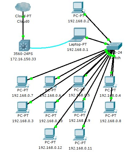
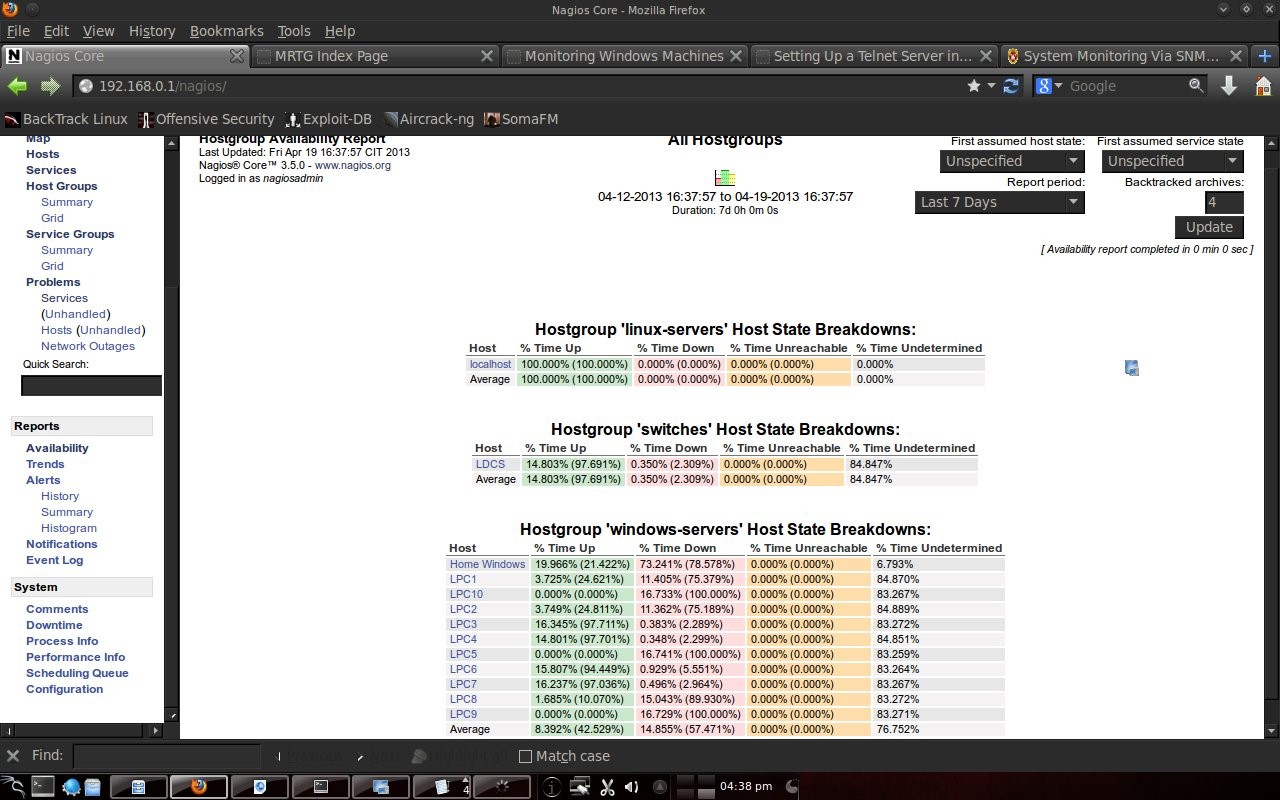
Nagios server is a laptop with IP 192.168.0.1. IP 192.168.0.2 and 192.168.0.3 are PCs with Ubuntu lts 12.04 operating system. The other PC is the Windows Tiny XP operating system. For all PCs have a default gateway of 192.168.0.1. The laptop will forward to 172.16.150.33. The laptop uses IP forward and iptables to forward to 172.16.150.33. Chapter 4 Discussion4.1 Nagios Display on browser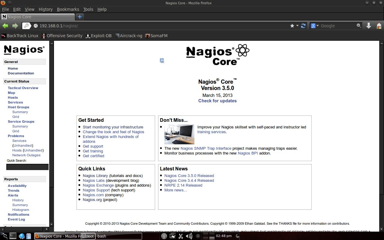
On the local network, Nagios can be accessed at the address http://192.168.0.1/nagios with the username Nagiosadmin and the password for Nagios. If you have a public IP and domain name, Nagios can be accessed with a domain address. 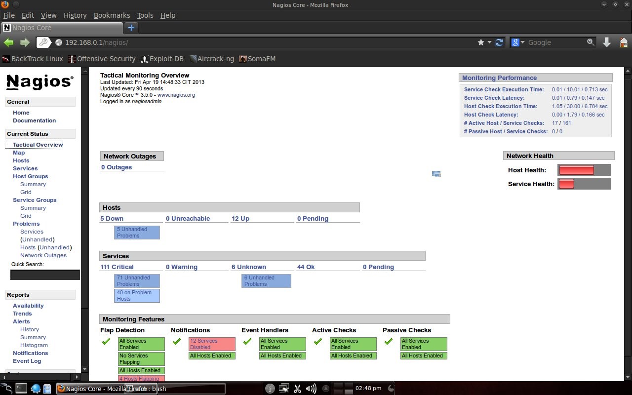
4.2 Host state display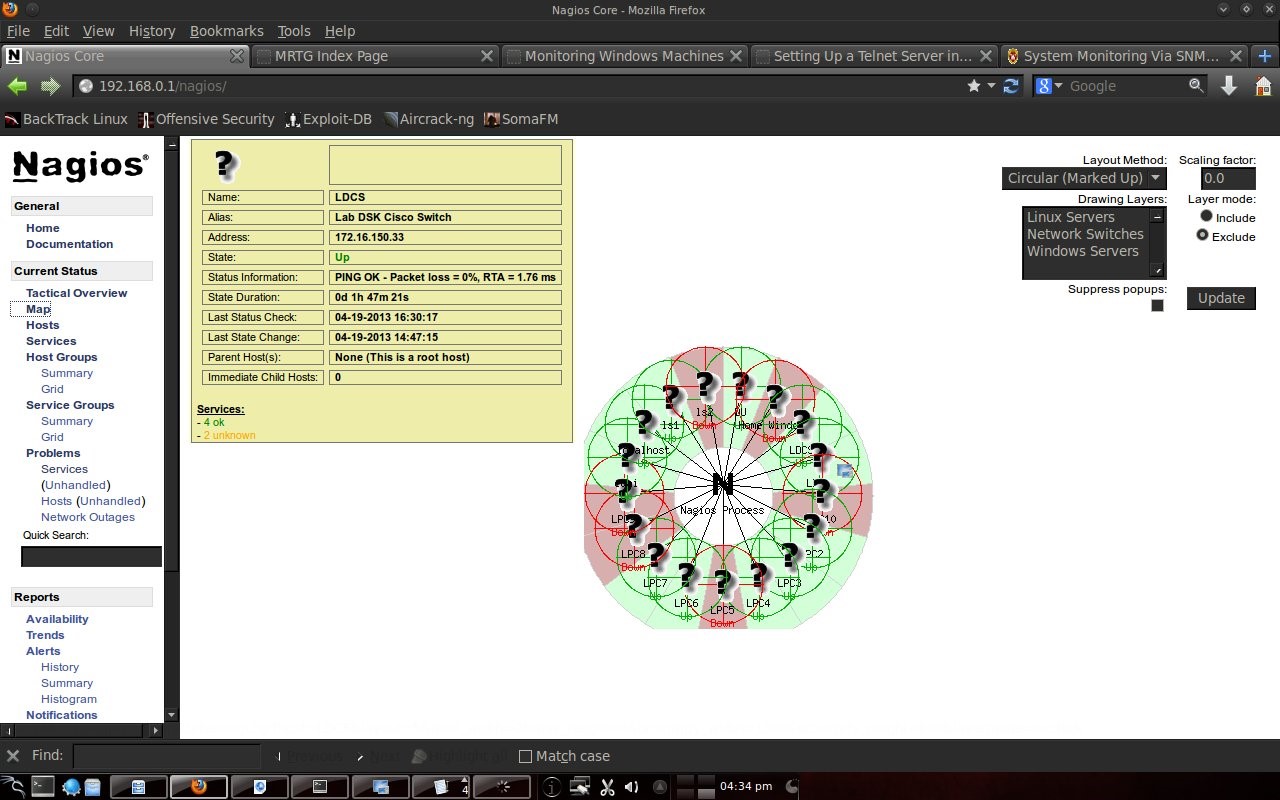
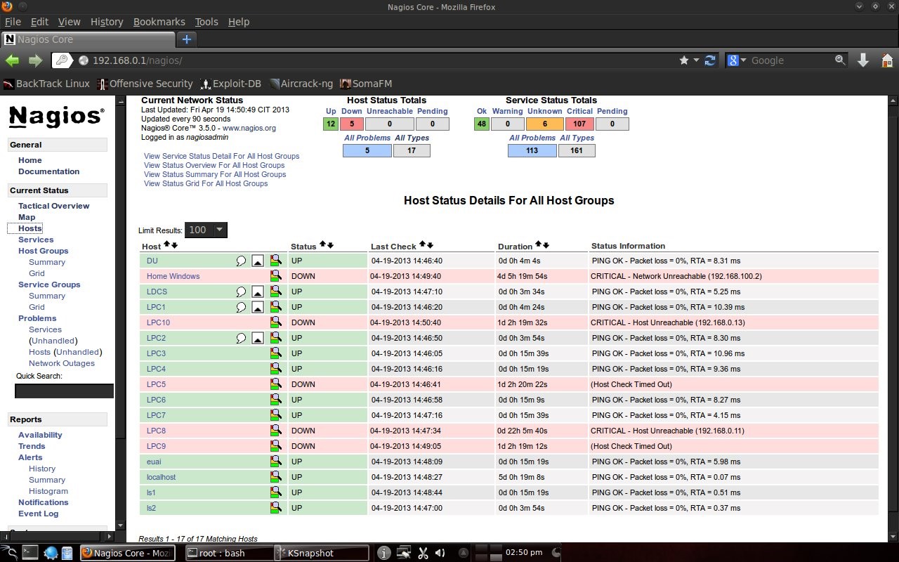
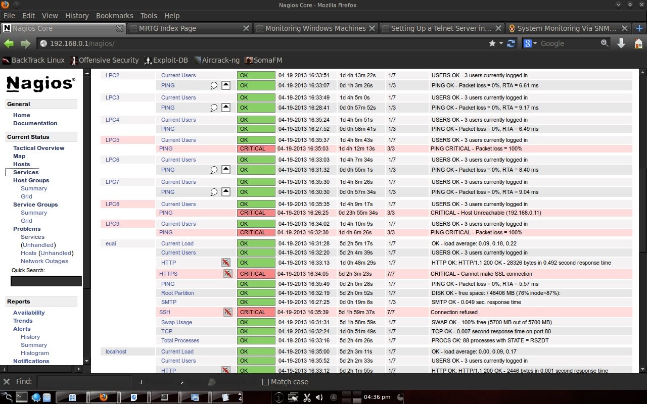
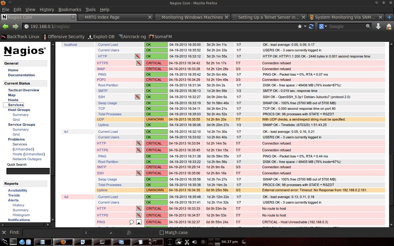
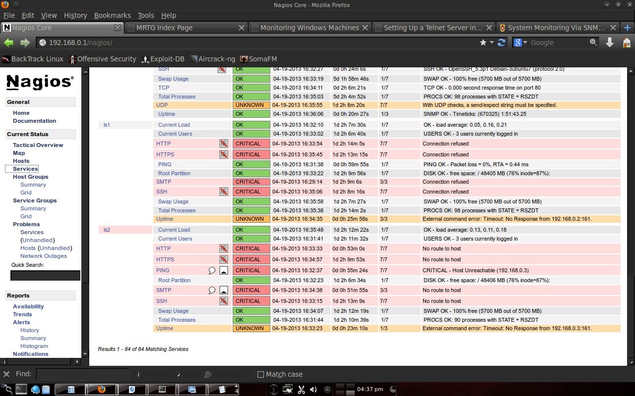
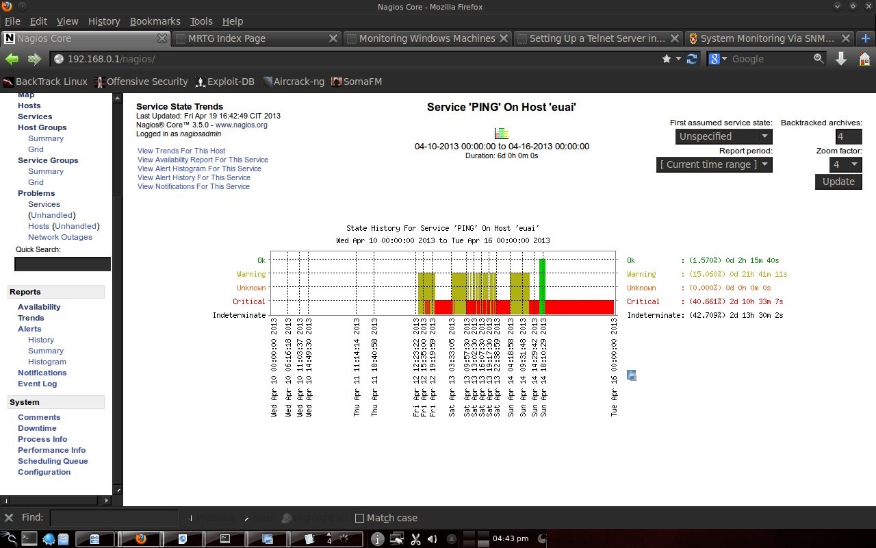
Here you can see that Home Windows is in a dead state because it is a computer in the author's house and is not connected to the computer lab. PC5, PC8, PC9 and PC10 labkom networks are off. After checking the physical condition, it turned out that there was a problem with the network cable. After the cable is replaced, the PC network is alive. The other hosts are normal. DU is DNS UNUD with IP 172.16.0.6, LDCS is Cisco Switch DSK Lab with IP 172.16.150.33, euai is elearning.unud.ac.id, ls is labkom server with Ubuntu linux operating system, and LPC is labkom PC with operating system Windows Tiny XP. 4.3 Service DisplayNagios can also monitor services on hosts such as http, smtp, ftp, dhcp, dns, mrtgtraf, partitions and others. Conditions are OK, warning, critical set by the user, for example ping, set a warning if the RTA (Round Trip Average) is above 200 ms and critical if it is above 300 ms. 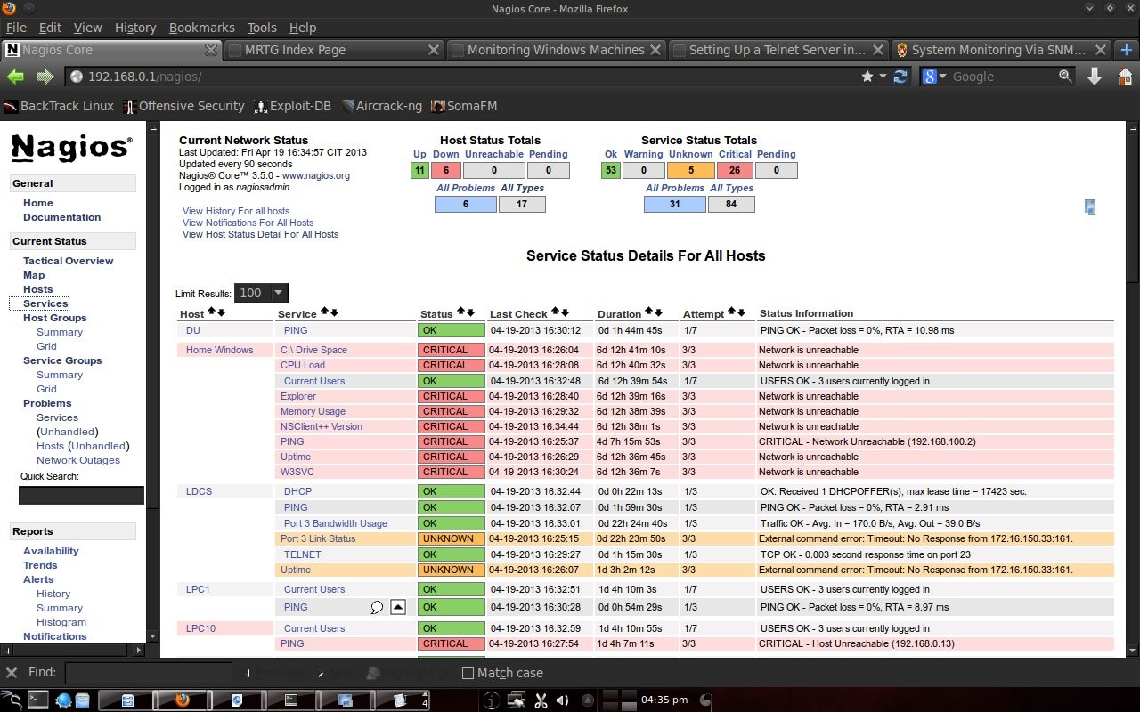
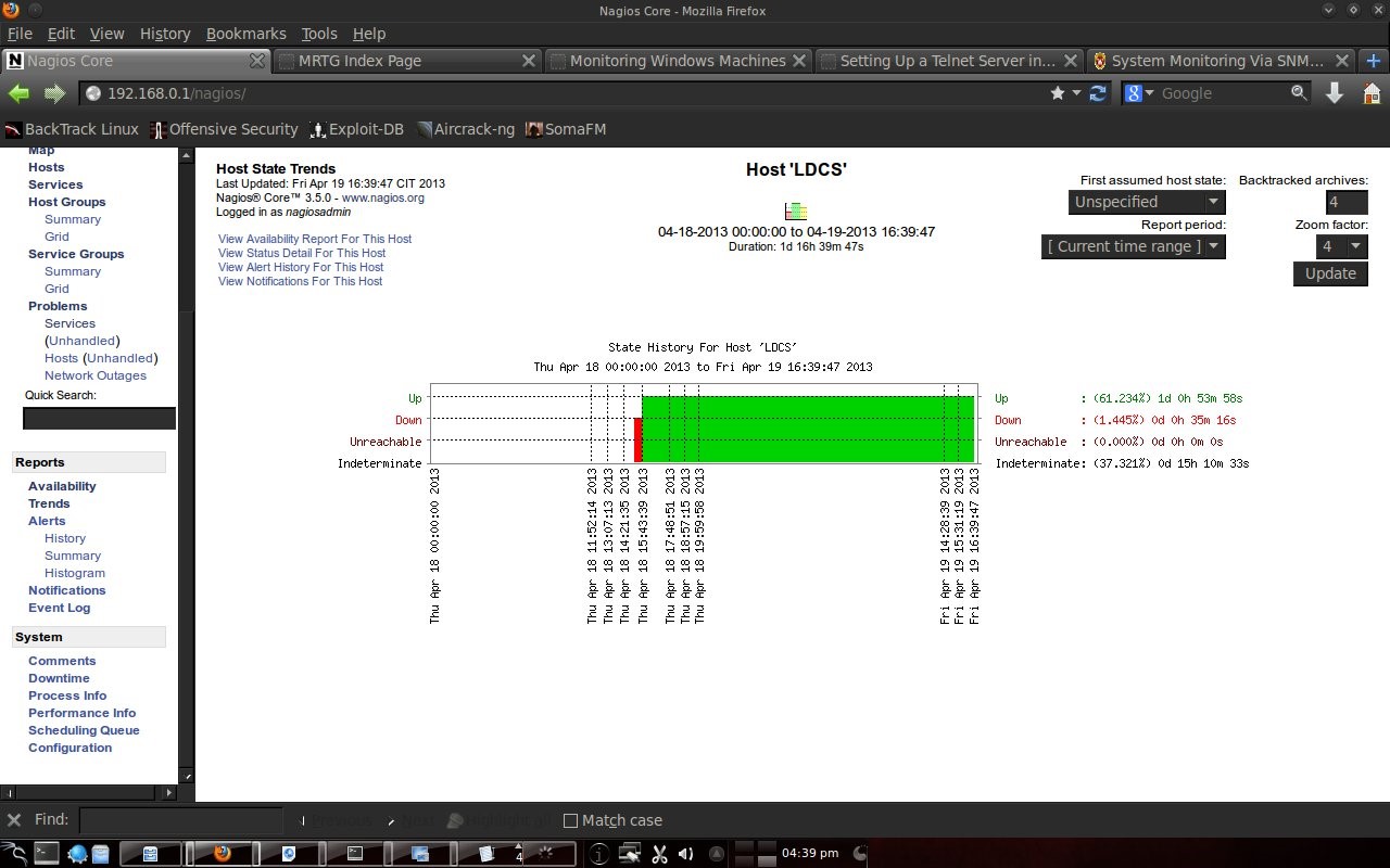
4.4 Report on NagiosNagios is also capable of making reports. What is reported is the host state from the first monitoring to the last condition. So the monitoring results were recorded by Nagios. 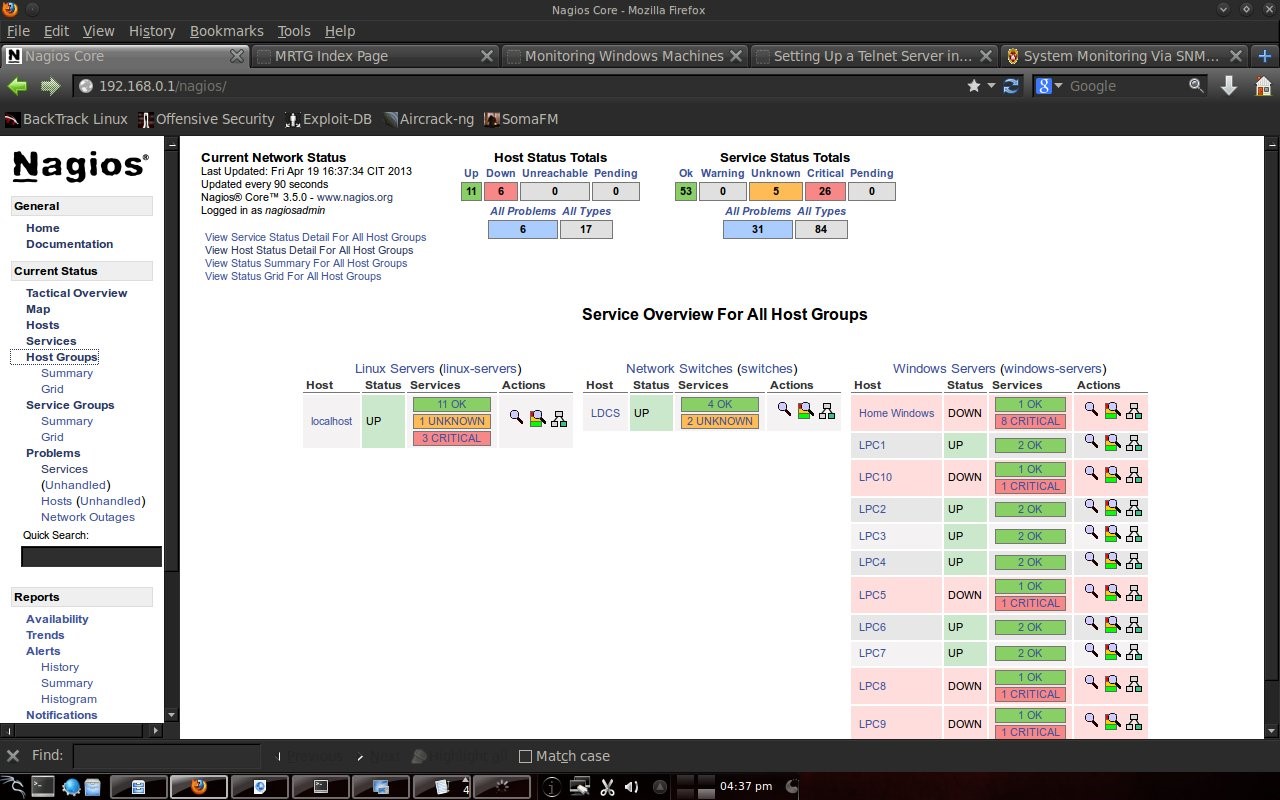
Chapter 5 Closing5.1 ConclusionIn the computer lab, Electrical Engineering, Udayana University is very suitable for installing Nagios (monitoring servers). With many PCs that are alive and used every day for almost 24 hours, Nagios can monitor the condition of the PC. Network to the Internet in the computer lab using the facilities of Udayana University. By being given a default gateway in the DSK lab and DNS UNUD, Nagios can monitor this. In trouble conditions, instead of checking devices 1 by 1 it is more efficient to see the state of the host with Nagios, because Nagios can display which ones are in good condition and which are in bad condition. Bibliography
Mirror
CatatanArtikel ini merupakan tugas dari mata kuliah Kehandalan Sistem Telekomunikasi S1 saya mengenai aplikasi Nagios yang dapat memantau keadaan jaringan komputer. Kebetulan saat itu saya juga asisten laboratium komputer. Sehingga saya dapat kesempatan untuk menerapkan Nagios di lab tersebut. Tugas ini tidak pernah dipublikasi dimanapun dan saya sebagai penulis dan pemegang hak cipta melisensi tulisan ini customized CC-BY-SA dimana siapa saja boleh membagi, menyalin, mempublikasi ulang, dan menjualnya dengan syarat mencatumkan nama saya sebagai penulis dan memberitahu bahwa versi asli dan terbuka ada disini. BAB 1 Pendahuluan1.1 Latar BelakangNagios suatu server untuk memantau keaadaan jaringan. Pada umumnya yang dipantau adalah host menggunakan service-service seperti check_ping, check_uptime, check_mrtgtraf dan service-service lainnya. Keunggulan pada nagios adalah pemantauannya dapat dilihat melalui halaman web (melalui port 80 http). Sehingga pemantau dapat memantau dari jarak jauh. Kini nagios core telah mencapai versi 3.5 dan nagios plugin 1.6. Nagios telah mendukung semua distribusi Linux, tetapi belum mendukung untuk Windows. Selain itu disediakan tutorial installasi dan langkah-langkah awal di situs web resmi nagios. Awalnya penulis belum pernah menggunakan nagios untuk memantau. Penulis berkeinginan untuk mengetahui bagaimana kualitas nagios menurut padangan penulis secara pribadi. Untuk bahan pemantauan disediakan 10 komputer dan 1 switch di laboratorium komputer, Teknik Elektro, Universitas Udayana. Pada percobaan ini akan dicoba menggunakan nagios untuk memantau 10 komputer dan 1 switch di labkom, selain itu juga memantau diri sendiri (localhost) dan 1 linux server melalui jaringan Internet, yaitu https://elearning.unud.ac.id 1.2 Rumusan MasalahBagaimana kualitas menurut pandangan secara pribadi penggunaan nagios untuk memonitor komputer dan switch di lab komputer, Teknik Elektro, Universitas Udayana? 1.3 TujuanMengetahui bagaimana penggunaan nagios di lab komputer, Teknik Elektro, Universitas Udayana. 1.4 Manfaat
1.5 Ruang Lingkup dan Batasan
BAB 2 Tinjauan Pustaka2.1 NagiosNagios adalah sistem pemantauan yang kuat yang memungkinkan organisasi untuk mengidentifikasi dan menyelesaikan masalah IT infrastruktur sebelum mereka mempengaruhi proses bisnis penting. Pertama kali diluncurkan pada tahun 1999, nagios telah berkembang untuk memasukkan ribuan proyek yang dikembangkan oleh komunitas nagios seluruh dunia. Nagios secara resmi disponsori oleh nagios Enterprises, yang mendukung masyarakat dalam sejumlah cara yang berbeda melalui penjualan produk dan layanan komersial. Nagios memonitor seluruh infrastruktur TI untuk memastikan sistem, aplikasi, layanan, dan proses bisnis yang berfungsi dengan baik. Dalam hal kegagalan, nagios dapat mengingatkan staf teknis dari masalah, yang memungkinkan mereka untuk memulai proses remediasi sebelum mempengaruhi proses bisnis, pengguna akhir, atau pelanggan. Dengan Nagios tidak akan pernah meninggalkan harus menjelaskan mengapa pemadaman infrastruktur terlihat menyakiti bottom line organisasi (Nagios, 2013). 2.2 PingPing adalah nama dari sebuah utilitas perangkat lunak standar (tool) digunakan untuk menguji koneksi jaringan. Hal ini dapat digunakan untuk menentukan apakah perangkat remote (seperti Web atau server game) dapat dicapai melalui jaringan dan, jika demikian, latency koneksi ini. Alat Ping adalah bagian dari Windows, Mac OS X dan Linux serta beberapa router dan konsol game. Kebanyakan alat ping menggunakan Internet Control Message Protocol (ICMP). Mereka mengirim pesan permintaan ke alamat jaringan target secara berkala dan mengukur waktu yang dibutuhkan untuk pesan respon tiba. Alat-alat ini biasanya mendukung opsi seperti, berapa kali untuk mengirim permintaan, seberapa besar pesan permintaan untuk mengirim, berapa lama untuk menunggu untuk setiap jawaban. Output dari ping bervariasi tergantung pada alat. Hasil standar termasuk, alamat IP komputer yang merespons, jangka waktu (dalam milidetik) antara mengirim permintaan dan menerima respon, indikasi berapa banyak jaringan hop antara meminta dan menanggapi komputer, pesan kesalahan jika komputer target tidak merespon (Mitchell, 2013). BAB 3 Metode dan Materi3.1 Tempat dan WaktuPercobaan dilakukan di Lab Komputer, Teknik Elektro, Universitas Udayana pada tanggal 13 April 2013 sampai 19 April 2013. 3.2 Alat
3.3 Bahan
3.4 Cara3.4.1 Instalasi NagiosInstalasi nagios dapat dilihat di http://nagios.sourceforge.net/docs/3_0/quickstart-ubuntu.html 3.4.2 Mengatur NagiosContoh pengaturan nagios dapat dilihat di http://nagios.sourceforge.net/docs/3_0/monitoring-routers.html. 3.4.3 Instalasi MRTGInstalasi MRTG dapat dilihat di https://help.ubuntu.com/community/MRTG. 3.4.4 Mengatur Koneksi Jaringan
Nagios server adalah laptop dengan IP 192.168.0.1. IP 192.168.0.2 dan 192.168.0.3 adalah PC dengan sistem operasi Ubuntu lts 12.04. Sedangkan PC lainnya adalah sistem operasi Windows Tiny XP. Untuk semua PC memiliki default gateway 192.168.0.1. Laptop akan meneruskan ke 172.16.150.33. Laptop menggunakan IP forward dan iptables untuk meneruskan ke 172.16.150.33. BAB 4 Pembahasan4.1 Tampilan nagios di browser
Di jaringan lokal nagios dapat diakses dengan alamat http://192.168.0.1/nagios dengan username nagiosadmin dan password nagios. Jika memiliki IP public dan domain name maka nagios dapat diakses dengan alamat domain.
4.2 Tampilan keadaan host
Disini terlihat bahwa Home Windows dalam keadaan mati karena merupakan komputer di rumah penulis dan tidak terkoneksi di lab komputer. Jaringan labkom PC5, PC8, PC9 dan PC10 dalam keadaan mati. Setelah diperiksa keadaan fisiknya ternyata ada masalah dengan kabel jaringannya. Setelah kabel tersebut diganti maka jaringan PC tersebut hidup. Host yang lain dalam keadaan normal. DU merupakan DNS UNUD dengan IP 172.16.0.6, LDCS adalah Lab DSK Cisco Switch dengan IP 172.16.150.33, euai adalah elearning.unud.ac.id, ls adalah labkom server dengan sistem operasi linux Ubuntu, dan LPC adalah labkom PC dengan sistem operasi Windows Tiny XP. 4.3 Tampilan ServiceNagios juga dapat memantau service pada host seperti http, smtp, ftp, dhcp, dns, mrtgtraf, partisi dan lain-lain. Kondisi OK, warning, critical diatur oleh user, contohnya ping, diatur warning jika RTA (Round Trip Average) diatas 200 ms dan critical jika diatas 300 ms.
4.4 Laporan pada nagiosNagios juga mampu membuat laporan. Hal yang dilaporkan adalah keadaan host dari pertama kali pemantauan hingga kondisi terkahir. Jadi hasil pemantauan dicatat oleh nagios.
BAB 5 Penutup5.1 SimpulanDi lab komputer, Teknik Elektro, Universitas Udayana sangat cocok untuk dipasangkan nagios (monitoring server). Dengan PC yang banyak yang hidup dan digunakan setiap hari hampir 24 jam maka nagios dapat memantau kondisi PC tersebut. Jaringan ke Internet di lab komputer menggunakan fasilitas dari Universitas Udayana. Dengan diberi default gateway di lab DSK dan DNS UNUD maka nagios dapat memantau hal tersebut. Pada kondisi trouble, Dari pada memeriksa perangkat 1 per 1 lebih effisien melihat keadaan host dengan nagios, karena nagios dapat menampilkan yang mana dalam keadaan baik dan yang dalam keadaan buruk. Daftar Pustaka
Mirror
If even famous crypto Youtubers said "what is this yield farming craziness? it is just putting your tokens and get a new token with fancy food names, the only reason they have value is because people speculates into them and when it ends then it will go back down", then what would regular people who even still doubts the future of Bitcoin thinks? This is a homework for everyone in DeFi farming if we want crops with sustainable value in the future. For those of you who are new to DeFi or yield farming, let us return to few prerequisite information before diving into the discussion. Does The Current DeFi Guarantees Full Ownership? What is Yield Farming 
If you think that process is complicated, then know that is actually still categorized as a very easy strategy. High yield DeFi farming can be more complicated. With the current gas fee system and demand, many people claimed that DeFi farming will only profitable when investing above $1000. Below that is not recommended except for just wanting to try. Before proceeding to the next section, here are todays famous farming platforms based on https://academy.binance.com/en/articles/what-is-yield-farming-in-decentralized-finance-defi: Compound FinanceCustomers needs to borrow tokens, Compound Finance requires suppliers and that could be us, we lend liquidity and Compound Finance rewards us in COMP tokens. Today, compound is one of the core protocol of yield farming ecosystem. MakerDAOWe lock assets as collateral to maintain the DAI token stable to one dollar. SynthetixSimilar to MakerDAO, we lock assets as collateral to issue tokens of anything that has price feed for example commodities, equities, and forex. AaveAnother lending and borrowing protocol but famous for its flash loans. Lenders get “aTokens†in return for their funds. UniswapThe most popular decentralized exchange (DEX) today using automated market maker (AAM). Supplier provides liquidity by locking their assets for customers to exchange tokens. Other than receiving commissions, suppliers receives UNI tokens Curve FinanceCurve Finance is a decentralized exchange protocol specifically designed for efficient stablecoin swaps. BalancerLike Uniswap liquidity provider but allows custom allocations while Uniswap allocations are only 50/50 for each exchange pair. Suppliers receives BAL token. Yearn FinanceYearn.finance is a decentralized ecosystem of aggregators for lending services such as Aave, Compound, and others. It aims to optimize token lending by algorithmically finding the most profitable lending services. Enter Harvest Finance  The Crops Utility
I did not hear any other utilities, if any of you know more, please mention them in the comment section. However, I know other utilities for other crypto coins:
Leave a comment for not only other utilities you know but also future utilities ideas. This is the homework for yield providers. As for Harvest Finance and other similiar platforms, the current strategy is to find the highest yield in price and/or quantity. There is an open room in developing strategies for determining other crop qualities. For example other than taking the utilities into account, a strategy can also be based on chain analysis such as number of holding address and amount of transactions, and another one is sentiment analysis. This way, we can also find undervalued crops. I am sure that most people preferred farming crops in increasing trend rather than crops in high volatility and/or decreasing trend. However, is it worth developing this feature now? I am not sure, because I am not sure with the crops utilities itself where the yield providers must provide value first but stashing this idea and take it into consideration in the future may proof advantageous. Disclaimer: most of the images are modifications from Harvest Finance and https://publicdomainvectors.org. Mirrors
NoteThis is English translated of my undergraduate assignment in Wireless Network course at the Department of Electrical Engineering, Faculty of Engineering, Udayana University. This assignment has never been published anywhere and I, as the author and copyright holder, license this assignment as customized CC-BY-SA where anyone can share, copy, republish, and sell on condition to state my name as the author and notify that the original and open version available here. Chapter 1 Introduction1.1 BackgroundThe signal strength received on the MS (Mobile Station) from the BS (Base Station) is generally affected at 3 stages. The first stage is signal generation at the BS (Base Station), the second stage is propagation, and the third stage is the MS (Mobile Station). Until now, there has not been an empirical calculation of signal propagation, which is currently used is prediction based on experiment and research (no theory). One of them is Okumura-Hata where researchers from Japan surround urban, suburban, and rural areas, trying certain distances and measuring the signal obtained by MS (Mobile Station) from BS (Base Station). To measure signal strength using Okumura must provide many tables based on the situation of the area. Even though using Okumura is accurate, it wastes time because we have to check the tables. Hata derived the calculation formula from Okumura but it also took a long time to compute manually. In this paper, calculations will be made from BS (Base Station) to MS (Mobile Station) based on the Hata formula in MATLAB software based on some data. What is calculated is the RX (Received) Power at MS (Mobile Station) in Urban, Suburban, and Rural areas from a distance of 1 km to 20 km. 1.2 ProblemWhat are the results of the calculation of receiver power in MS (Mobile Station) from transmitter BS (Base Station) in urban, suburban, and rural areas based on the Hata formula using MATLAB software? 1.3 ObjectiveTo make signal propagation calculations from BS (Base Station) to MS (Mobile Station) based on Okumura-Hata in MATLAB. 1.4 BenefitIt is more energy and time efficient to find signal propagation calculations. 1.5 Scope and Limits
Chapter 2 Literature Review2.1 Signal StrengthThe unit of signal strength is the watt, which is the unit of power in electricity. To facilitate the calculation of the signal strength from watts it is converted into decibell units (Kolawole, 2002). Where: P = Electrical power (watt)2.2 Free Space Loss Free Space Loss is the signal strength loss in a vacuum, depending on wavelength and distance. This is a loss that must exist (Kolawole, 2002). Where: FSL = Free Space Loss r = the distance between the transmitter and the receiver (meter) lamda = wavelength (meter) c = speed of light (meter/second) 2.3 Hata Path LossUntil now, the empirical formula for calculating the signal strength from BS (Base Station) to MS (Mobile Station) has not been found in the real world environment. What does exist is an approximate prediction based on research. Okumura and Hata surround an area at certain intensities and record the signal strength received by the MS (Mobile Station) from the BS (Base Station) at certain distances. The calculation of the Hata model is as follows (ETSI, 1999): Limitation: Frequency (f): 150 - 1000 MHz Base Station Height (Hb): 30 - 200 m Mobile Height (Hm): 1 - 10 m Distance (d): 1 - 20 km Untuk wilayah metropolitan: a(Hm)= f ≤ 200 MHz a(Hm)= f ≥ 400 MHz For nonmetropolitan areas: a(Hm)= Loss for Urban area: 6.55log(Hb)log(d) Loss for Suburban area Loss for Rural Quasi-Open area Loss for Rural Open-Area 2.4 Link BudgetIn general, there are 3 steps to calculate the signal strength from the BS (Base Station) to the MS (Mobile Station). The first stage is the signal strength generated by the BS (Base Station) affected by the smear loss and gain that occurs at the BS (Base Station). The second stage is the path loss, it can be calculated with Hata. The third stage is the gain and loss that occurs in MS (Mobile Station). Therefore it can be calculated (ETSI, 1999): Where: Pm = Signal strength on MS Pb = Signal strength on BS Gb = Gain Atenna BS Ld = Duplexer Loss BS Lj = Jumper Loss BS Lf = Feeder Loss BS Ltf = Filter Loss BS Mf = Fade Margin Ab = Body Atennuation Av = Vehide Atennuation Abd = Building Atennuation Lpj = Path loss Lm = Feeder Loss MS Gm = Gain Atenna MS Lo = Other Loss 2.5 MATLABMATLAB is a high-level language and an interactive environment for numerical computation, visualization, and programming. Using MATLAB, you can analyze data, develop algorithms, and create models and applications. Languages, tools, and built-in math functions allow you to explore multiple approaches and reach solutions faster than traditional spreadsheets or programming languages, such as C / C ++ or Java. MATLAB can be used for a wide variety of applications, including signal processing and communications, image and video processing, control systems, test and measurement, computational finance, and computational biology. More than one million engineers and scientists in industry and academia use MATLAB, the language of technical computing (Little, 2013). Chapter 3 Experimental Method3.1 Place and Time of ExperimentThe experiment was carried out at home on May 22, 2013. 3.2 Tools3.3 ProgramCreated 3 programs. The first program to calculate the path loss according to Hata for urban, suburban, and rural areas with distances of 1km, 2km, 3km, 4km, 5km, 6km, 7km, 8km, 9km, 10km, 11km, 12km, 13km, 14km, 15km, 16km, 17km, 18km, 19km, 20km. The second program is product loss, which is the sum of the path loss and indoor propagation loss. The third program for calculating the RX signal strength based on TX, gain, and loss on the device. Can also be made in simulink. 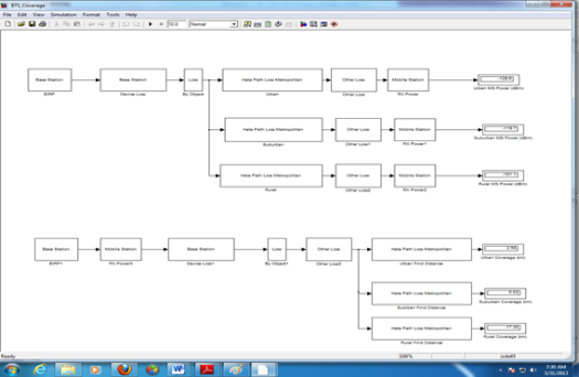
%Hata Model%Frequency 150 – 1000 (MHz)
f = 900;

%Base station height 30 – 200 (m)
Hb = 40;

%Mobile Height 1 – 10 (m)
Hm = 1.5;

%Distance 1 – 20 (km)
d = 1:20;

%Urban Area Loss small medium city (dB)
asm = (((1.1*log10(f))-0.7)*Hm)-((1.56*log10(f))-0.8);
Lusm = 69.55 + (26.16*log10(f)) – (13.82*log10(Hb)) – asm + ((44.9 – (6.55*log10(Hb)))*log10(d));

%Urban Area Loss large city (dB)
if f <= 200
    al = (8.29*(log10(1.54*Hm).^2))-1.1;
    Lul = 69.55 + (26.16*log10(f)) – (13.82*log10(Hb)) – al + ((44.9 – (6.55*log10(Hb)))*log10(d));
else if f >= 400
    al = (3.2*(log10(11.75*Hm).^2))-4.97;
    Lul = 69.55 + (26.16*log10(f)) – (13.82*log10(Hb)) – al + ((44.9 – (6.55*log10(Hb)))*log10(d));
else
    ‘frequency range undefine’;
end

%Suburban Area Loss small medium city (dB)
Lsusm = Lusm – (2*(log10(f/28).^2))-5.4;

%Suburban Area large city (dB)
Lsul = Lul – (2*(log10(f/28).^2))-5.4;

%Rural Area small medium city (Quasi-Open) (dB)
Lrqosm = Lusm – (4.78*(log10(f).^2))+(18.33*log10(f))-35.94;

%Rural Area large city (Quasi-Open) (dB)
Lrqol = Lul – (4.78*(log10(f).^2))+(18.33*log10(f))-35.94;

%Rural Area small medium city (Open Area) (dB)
Lrosm = Lusm – (4.78*(log10(f).^2))+(18.33*log10(f))-40.94;

%Rural Area large city (Open Area) (dB)
Lrol = Lul – (4.78*(log10(f).^2))+(18.33*log10(f))-40.94;

subplot(2,1,1);
plot(d,Lusm,d,Lsusm,d,Lrqosm,d,Lrosm);
grid on;
subplot(2,1,2);
plot(d,Lul,d,Lsul,d,Lrqol,d,Lrol);
grid on;
Code 3.1 Path Loss Hata Model %Product Loss%u = urban %s = surban %r = rural %Total Path Loss (dB) Lptu = Lul; Lpts = Lsul; Lptr = Lrol; %Building Attenuation (dB) Abdu = 15; Abds = 12; Abdr = 0; %Vhide Attenuation (dB) Avu = 0; Avs = 0; Avr = 0; %Body Attenuation (dB) Abu = 2; Abs = 2; Abr = 2; %Fade Margin (dB) Mfu = 5.6; Mfs = 5.6; Mfr = 5.6; %Feeder loss per meter (dB/m) Lf_m = 0.0646; %Feeder loss (dB) Lf = Hb*Lf_m; %Product Loss (dB) Lpu = Lptu + Abdu + Avu + Abu + Mfu + Lf; Lps = Lpts + Abds + Avs + Abs + Mfs + Lf; Lpr = Lptr + Abdr + Avr + Abr + Mfr + Lf; Code 3.2 Product Loss %MS_BS RX Power%u = urban %s = surban %r = rural %MS TX Power (dBm) Pm = 30; %MS Antenna Gain (dBi) Gm = 2; %MS Feeder Loss (dB) Lm = 0; %BS TX Power (dBm) Pb = 47; %BS Antenna Gain (dBi) Gb = 20; %BS Diversity Gain (dB) Gd = 3.5; %BS Duplexer Loss (dB) Ld = 0.8; %BS Jumper/Connector Loss (dB) Lj = 0.9; %BS TX Filter Loss (dB) Ltf = 2.3; %Other Loss (dB) Lo = 0; %BS RX Power Sbu = Pm + Gm – Lm + Gb + Gd – Ld – Lj – Lpu – Lo; Sbs = Pm + Gm – Lm + Gb + Gd – Ld – Lj – Lps – Lo; Sbr = Pm + Gm – Lm + Gb + Gd – Ld – Lj – Lpr – Lo; %MS RX Power Smu = Gm – Lm + Pb + Gb – Ld – Lj – Ltf – Lpu – Lo; Sms = Gm – Lm + Pb + Gb – Ld – Lj – Ltf – Lps – Lo; Smr = Gm – Lm + Pb + Gb – Ld – Lj – Ltf – Lpr – Lo; plot(d,Smu,d,Sms,d,Smr); legend(‘Urban’, ‘Suburban’, ‘Rural’); title(‘Received Power’); xlabel(‘Distance (km)’); ylabel(‘Power (dBm)’); grid on; Code 3.3 BS MS Power
a = 20; b = 20; ang=0:0.01:2*pi;
x1=d(1)*cos(ang);
y1=d(1)*sin(ang);
x2=d(2)*cos(ang);
y2=d(2)*sin(ang);
x3=d(3)*cos(ang);
y3=d(3)*sin(ang);
x4=d(4)*cos(ang);
y4=d(4)*sin(ang);
x5=d(5)*cos(ang);
y5=d(5)*sin(ang);
x6=d(6)*cos(ang);
y6=d(6)*sin(ang);
x7=d(7)*cos(ang);
y7=d(7)*sin(ang);
x8=d(8)*cos(ang);
y8=d(8)*sin(ang);
x9=d(9)*cos(ang);
y9=d(9)*sin(ang);
x10=d(10)*cos(ang);
y10=d(10)*sin(ang);
x11=d(11)*cos(ang);
y11=d(11)*sin(ang);
x12=d(12)*cos(ang);
y12=d(12)*sin(ang);
x13=d(13)*cos(ang);
y13=d(13)*sin(ang);
x14=d(14)*cos(ang);
y14=d(14)*sin(ang);
x15=d(15)*cos(ang);
y15=d(15)*sin(ang);
x16=d(16)*cos(ang);
y16=d(16)*sin(ang);
x17=d(17)*cos(ang);
y17=d(17)*sin(ang);
x18=d(18)*cos(ang);
y18=d(18)*sin(ang);
x19=d(19)*cos(ang);
y19=d(19)*sin(ang);
x20=d(20)*cos(ang);
y20=d(20)*sin(ang);

%plot(a+x1,b+y1,a+x2,b+y2,a+x3,b+y3,a+x4,b+y4,a+x5,b+y5,a+x6,b+y6,a+x7,b+y7,a+x8,b+y8,a+x9,b+y9,a+x10,b+y10,a+x11,b+y11,a+x12,b+y12,a+x13,b+y13,a+x14,b+y14,a+x15,b+y15,a+x16,b+y16,a+x17,b+y17,a+x18,b+y18,a+x19,b+y19,a+x20,b+y20);
fill(a+x20,b+y20,[0.4 0 0],a+x19,b+y19,[0.6 0 0],a+x18,b+y18,[0.9 0 0],a+x17,b+y17,[1 0.2 0],a+x16,b+y16,[1 0.4 0],a+x15,b+y15,[1 0.7 0],…
a+x14,b+y14,[1 0.9 0],a+x13,b+y13,[0.8 1 0],a+x12,b+y12,[0.6 1 0],a+x11,b+y11,[0 1 0.3],a+x10,b+y10,[0 1 0.5],a+x9,b+y9,[0 1 0.7],…
a+x8,b+y8,[0 1 0.9],a+x7,b+y7,[0 1 1],a+x6,b+y6,[0 0.7 1],a+x5,b+y5,[0 0.6 1],a+x4,b+y4,[0 0.4 1],a+x3,b+y3,[0 0.3 1],…
a+x2,b+y2,[0 0.2 1],a+x1,b+y1,[0 0 1]);
colorbar(‘YTickLabel’,{‘0’,Smu(2),Smu(4),Smu(6),Smu(8),Smu(10),Smu(12),Smu(14),Smu(16),Smu(18),Smu(20)});
grid on;
xlabel(‘X-distance (km)’); %# Add an x axis label
ylabel(‘Y-distance (km)’); %# Add a y axis label
subplot(3,1,1);
Code 3.4 Coverage 1/2
fill(a+x20,b+y20,[0.4 0 0],a+x19,b+y19,[0.6 0 0],a+x18,b+y18,[0.9 0 0],a+x17,b+y17,[1 0.2 0],a+x16,b+y16,[1 0.4 0],a+x15,b+y15,[1 0.7 0],…a+x14,b+y14,[1 0.9 0],a+x13,b+y13,[0.8 1 0],a+x12,b+y12,[0.6 1 0],a+x11,b+y11,[0 1 0.3],a+x10,b+y10,[0 1 0.5],a+x9,b+y9,[0 1 0.7],… a+x8,b+y8,[0 1 0.9],a+x7,b+y7,[0 1 1],a+x6,b+y6,[0 0.7 1],a+x5,b+y5,[0 0.6 1],a+x4,b+y4,[0 0.4 1],a+x3,b+y3,[0 0.3 1],…
a+x2,b+y2,[0 0.2 1],a+x1,b+y1,[0 0 1]);
colorbar(‘YTickLabel’,{‘0’,Smu(4),Smu(8),Smu(15),Smu(17),Smu(20)});
grid on;
xlabel(‘X-distance (km)’); %# Add an x axis label
ylabel(‘Y-distance (km)’); %# Add a y axis label
subplot(3,1,2);

fill(a+x20,b+y20,[0.4 0 0],a+x19,b+y19,[0.6 0 0],a+x18,b+y18,[0.9 0 0],a+x17,b+y17,[1 0.2 0],a+x16,b+y16,[1 0.4 0],a+x15,b+y15,[1 0.7 0],…
a+x14,b+y14,[1 0.9 0],a+x13,b+y13,[0.8 1 0],a+x12,b+y12,[0.6 1 0],a+x11,b+y11,[0 1 0.3],a+x10,b+y10,[0 1 0.5],a+x9,b+y9,[0 1 0.7],…
a+x8,b+y8,[0 1 0.9],a+x7,b+y7,[0 1 1],a+x6,b+y6,[0 0.7 1],a+x5,b+y5,[0 0.6 1],a+x4,b+y4,[0 0.4 1],a+x3,b+y3,[0 0.3 1],…
a+x2,b+y2,[0 0.2 1],a+x1,b+y1,[0 0 1]);
colorbar(‘YTickLabel’,{‘0’,Sms(4),Sms(8),Sms(15),Sms(17),Sms(20)});
grid on;
xlabel(‘X-distance (km)’); %# Add an x axis label
ylabel(‘Y-distance (km)’); %# Add a y axis label
subplot(3,1,3);

fill(a+x20,b+y20,[0.4 0 0],a+x19,b+y19,[0.6 0 0],a+x18,b+y18,[0.9 0 0],a+x17,b+y17,[1 0.2 0],a+x16,b+y16,[1 0.4 0],a+x15,b+y15,[1 0.7 0],…
a+x14,b+y14,[1 0.9 0],a+x13,b+y13,[0.8 1 0],a+x12,b+y12,[0.6 1 0],a+x11,b+y11,[0 1 0.3],a+x10,b+y10,[0 1 0.5],a+x9,b+y9,[0 1 0.7],…
a+x8,b+y8,[0 1 0.9],a+x7,b+y7,[0 1 1],a+x6,b+y6,[0 0.7 1],a+x5,b+y5,[0 0.6 1],a+x4,b+y4,[0 0.4 1],a+x3,b+y3,[0 0.3 1],…
a+x2,b+y2,[0 0.2 1],a+x1,b+y1,[0 0 1]);
colorbar(‘YTickLabel’,{‘0’,Smr(4),Smr(8),Smr(15),Smr(17),Smr(20)});
grid on;
xlabel(‘X-distance (km)’); %# Add an x axis label
ylabel(‘Y-distance (km)’); %# Add a y axis label
Code 3.5 Coverage 2/2 3.4 InputTable 3.2 Input 1
3.5 Output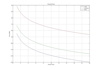

Chapter 4 Discussion4.1 Signal Strength in MS (Mobile Station)It can be seen in Figure 3.1 that the signal strength decreases exponentially with the distance between the MS (Mobile Station) and the BS (Base Station). According to Hata and Free Space Loss, the signal loss will get bigger as the distance value increases (d). A clearer graphic can be seen in Figure 4.1. 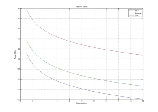%20diperbesar.png)
From the graph above, it can be seen that the Hata formula shows that urban MS (Mobile Station) has the lowest signal strength value compared to suburban and rural areas. Meanwhile, rural areas have the highest signal strength. If using the Hata formula at a distance of 20 km, the Mobile must have a minimum sensitivity of -130 dBm in urban areas, -117 dBm in suburban areas, and -86 dBm in rural areas. Using MATLAB can also illustrate the value of the MS signal strength in the form of a map at a certain radius as follows with the BS in the middle: 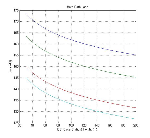
The graph and image above are the values: 6.55log(Hb))log(d) With input variations d = 1 km to d = 20 km. The formula above is Loss according to the Hata Model. The formula is based on the ETSI 1999 standard. 4.2 Increase MS Power4.2.1 Minimizes Hata Path LossAt first glance the Hata formula does not appear whether the frequency or high parameters of the BTS should be increased or decreased. The distance and height variables MS are natural so they cannot be adjusted. If you use MATLAB, you can see the effect of frequency and height of BTS on loss (with d = 20 km and Hm = 1.5 m). 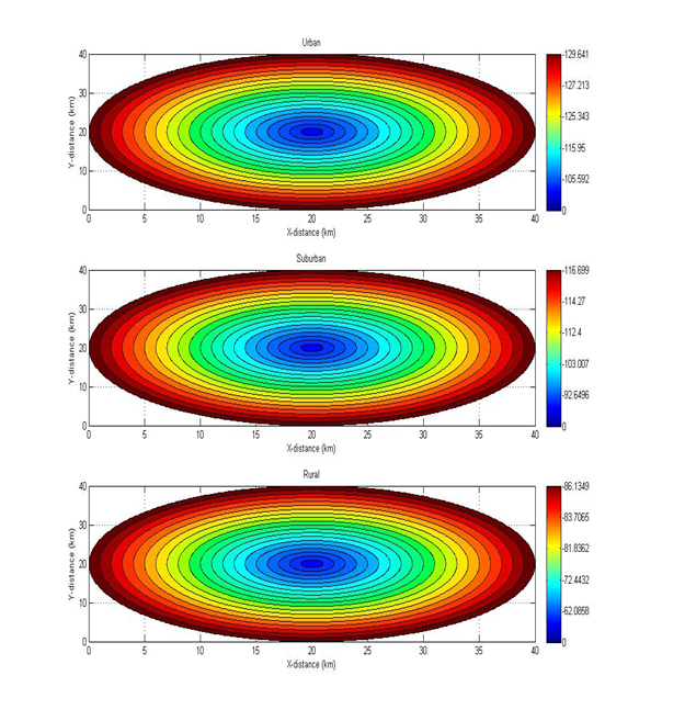
From the graph above, it can be seen that the Path Loss will decrease when the BS (Base Station) gets higher. Therefore increasing the BTS height is one solution to reduce loss. The graph above shows the values: 6.55log(Hb))log(d) With a variation of input Hb = 30 m to d = 200 m. The formula above is Loss according to the Hata Model. The formula is based on the ETSI 1999 standard. 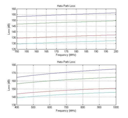
From the chart above, it can be seen that the Path Loss will increase the higher the frequency. The graph above shows the values: 6.55log(Hb))log(d) With input variations f = 150 MHz to f = 1000 MHz. The formula above is Loss according to the Hata Model. The formula is based on the ETSI 1999 standard. 4.2.2 Increasing Tool SpecificationsBased on the link budget formula from ETSI 1999: A higher MS (Mobile Station) signal strength value can be achieved by increasing antenna gain, increasing BS (Base Station) transmit power, and minimizing device loss. Chapter 5 Closing5.1 ConclusionUsing MATLAB is much faster than manual counting and can graph and illustrate a BS (Base Station) radius illustration with MS (Mobile Station). From the MATLAB results at a distance of 1 km, the signal strength of MS is -85 dBm in urban areas, -72 dBm in suburban areas, and -8-41 dBm in rural areas. At the farthest distance of 20 km, the signal strength of MS is -130 dBm in urban areas, -117 dBm in suburban areas, and -86 dBm in rural areas. Bibliography
CatatanTulisan ini merupakan tugas S1 mata kuliah Jaringan Nirkabel saya di Jurusan Teknik Elektro, Fakultas Teknik, Universitas Udayana. Tugas ini tidak pernah dipublikasi dimanapun dan saya sebagai penulis dan pemegang hak cipta melisensi tulisan ini customized CC-BY-SA dimana siapa saja boleh membagi, menyalin, mempublikasi ulang, dan menjualnya dengan syarat mencatumkan nama saya sebagai penulis dan memberitahu bahwa versi asli dan terbuka ada disini. BAB 1 Pendahuluan1.1 Latar BelakangKuat sinyal yang diterima pada MS (Mobile Station) dari BS (Base Station) dipengaruhi secara umum pada 3 tahap. Tahap pertama adalah pembangkitan sinyal pada BS (Base Station), tahap kedua adalah propagasi, dan tahap ketiga adalah MS (Mobile Station). Sampai saat ini belum ditemukan perhitungan secara empiris propagasi sinyal, yang digunakan saat ini adalah prediksi berdasarkan percobaan dan penelitian (tidak ada teori). Salah satunya adalah Okumura-Hata dimana peneliti dari Jepang mengelilingi daerah urban, suburban, dan rural, mencoba jarak – jarak tertentu dan mengukur sinyal yang didapatkan oleh MS (Mobile Station) dari BS (Base Station). Untuk mengukur kuat sinyal menggunakan Okumura harus menyediakan tabel yang banyak berdasarkan situasi daerah. Walaupun menggunakan Okumura akurat namun boros terhadap waktu karena harus mengecek tabel. Hata menurunkan rumus perhitungan dari Okumura tetapi juga memerlukan waktu yang lama untuk dihitung secara manual. Pada makalah ini akan dibuat perhitungan dari BS (Base Station) ke MS (Mobile Station) berdasarkan rumus Hata di software MATLAB berdasarkan suatu data. Yang dihitung adalah RX (Received) Power di MS (Mobile Station) di daerah Urban, Suburban, dan Rural dari jarak 1 km sampai 20 km. 1.2 Rumusan MasalahBagaimana hasil perhitungan daya receiver di MS (Mobile Station) dari transmitter BS (Base Station) di daerah urban, suburban, dan rural berdasarkan rumus Hata menggunakan software MATLAB? 1.3 TujuanUntuk membuat perhitungan propagasi sinyal dari BS (Base Station) ke MS (Mobile Station) berdasarkan Okumura-Hata di MATLAB. 1.4 ManfaatLebih effisien tenaga dan waktu untuk mencari perhitungan propagasi sinyal. 1.5 Ruang Lingkup dan Batasan
BAB 2 Tinjauan Pustaka2.1 Kuat SinyalSatuan kuat sinyal adalah watt yaitu satuan daya pada listrik. Untuk memudahkan perhitungan kuat sinyal dari satuan watt dikonversi menjadi satuan decibell (Kolawole, 2002). Dimana: P = Daya listrik (watt)2.2 Free Space Loss Free Space Loss adalah kehilangan kuat sinyal di ruang hampa, tergantung pada panjang gelombang dan jarak. Ini merupakan loss yang pasti ada (Kolawole, 2002). Dimana: FSL = Free Space Loss r = jarak antara transmitter dengan receiver (meter) lamda = panjang gelombang (meter) c = kecepatan cahaya (meter/second) 2.3 Hata Path LossSampai saat ini belum ditemukan rumus empiris perhitungan kuat sinyal dari BS (Base Station) ke MS (Mobile Station) pada lingkungan di dunia nyata. Yang ada adalah prediksi yang mendekati berdasarkan penelitian. Okumura dan Hata mengelilingi suatu daerah pada intensitas-intensitas tertentu dan mencatat kuat sinyal yang diterima MS (Mobile Station) dari BS (Base Station) pada jarak-jarak tertentu. Perhitungan Hata model sebagai berikut (ETSI, 1999): Syarat: Frequency (f): 150 - 1000 MHz Base Station Height (Hb): 30 - 200 m Mobile Height (Hm): 1 - 10 m Distance (d): 1 - 20 km Untuk wilayah metropolitan: a(Hm)= f ≤ 200 MHz a(Hm)= f ≥ 400 MHz Untuk wilayah nonmetropolitan: a(Hm)= Loss pada daerah Urban: 6.55log(Hb)log(d) Loss pada daerah Suburban Loss pada daerah Rural Quasi-Open Loss pada daerah Rural Open-Area 2.4 Link BudgetPerhitungan kuat sinyal dari BS (Base Station) ke MS (Mobile Station) secara umum ada 3 tahap. Tahap pertama adalah kuat sinyal yang dibangkitkan oleh BS (Base Station) dipengaruhi oles loss dan gain yang terjadi di BS (Base Station). Tahap kedua adalah path loss, dapat dihitung dengan Hata. Tahap ketiga adalah gain dan loss yang terjadi pada MS (Mobile Station). Oleh karena itu dapat dihitung (ETSI, 1999): Dimana: Pm = Kuat sinyal pada MS Pb = Kuat sinyal dibangkit pada BS Gb = Gain Atenna BS Ld = Duplexer Loss BS Lj = Jumper Loss BS Lf = Feeder Loss BS Ltf = Filter Loss BS Mf = Fade Margin Ab = Body Atennuation Av = Vehide Atennuation Abd = Building Atennuation Lpj = Path loss Lm = Feeder Loss MS Gm = Gain Atenna MS Lo = Other Loss 2.5 MATLABMATLAB adalah bahasa tingkat tinggi dan lingkungan yang interaktif untuk perhitungan numerik, visualisasi, dan pemrograman. Menggunakan MATLAB, dapat menganalisis data, mengembangkan algoritma, dan membuat model dan aplikasi. Bahasa, peralatan, dan built-in fungsi matematika memungkinkan Anda untuk menjelajahi beberapa pendekatan dan mencapai solusi lebih cepat dibandingkan dengan spreadsheet atau bahasa pemrograman tradisional, seperti C / C + + atau Java. MATLAB dapat digunakan untuk berbagai aplikasi, termasuk pemrosesan sinyal dan komunikasi, gambar dan video processing, sistem kontrol, uji dan pengukuran, keuangan komputasi, dan biologi komputasi. Lebih dari satu juta insinyur dan ilmuwan dalam industri dan akademisi menggunakan MATLAB, bahasa komputasi teknis (Little, 2013). BAB 3 Metode Percobaan3.1 Tempat dan Waktu PercobaanPercobaan dilakukan di Rumah pada tanggal 22 Mei 2013. 3.2 Alat3.3 ProgramDibuat 3 program. Program pertama untuk menghitung path loss menurut Hata pada daerah urban, suburban, dan rural dengan jarak 1km, 2km, 3km, 4km, 5km, 6km, 7km, 8km, 9km, 10km, 11km, 12km, 13km, 14km, 15km, 16km, 17km, 18km, 19km, 20km. Program kedua adalah product loss adalah penjumlahan path loss dengan loss propagasi indoor. Program ketiga untuk adalah perhitungan kuat sinyal RX berdasarkan TX, gain, dan loss pada perangkat. Dapat juga dibuat dalam simulink.
%Hata Model%Frequency 150 – 1000 (MHz)
f = 900;

%Base station height 30 – 200 (m)
Hb = 40;

%Mobile Height 1 – 10 (m)
Hm = 1.5;

%Distance 1 – 20 (km)
d = 1:20;

%Urban Area Loss small medium city (dB)
asm = (((1.1*log10(f))-0.7)*Hm)-((1.56*log10(f))-0.8);
Lusm = 69.55 + (26.16*log10(f)) – (13.82*log10(Hb)) – asm + ((44.9 – (6.55*log10(Hb)))*log10(d));

%Urban Area Loss large city (dB)
if f <= 200
    al = (8.29*(log10(1.54*Hm).^2))-1.1;
    Lul = 69.55 + (26.16*log10(f)) – (13.82*log10(Hb)) – al + ((44.9 – (6.55*log10(Hb)))*log10(d));
else if f >= 400
    al = (3.2*(log10(11.75*Hm).^2))-4.97;
    Lul = 69.55 + (26.16*log10(f)) – (13.82*log10(Hb)) – al + ((44.9 – (6.55*log10(Hb)))*log10(d));
else
    ‘frequency range undefine’;
end

%Suburban Area Loss small medium city (dB)
Lsusm = Lusm – (2*(log10(f/28).^2))-5.4;

%Suburban Area large city (dB)
Lsul = Lul – (2*(log10(f/28).^2))-5.4;

%Rural Area small medium city (Quasi-Open) (dB)
Lrqosm = Lusm – (4.78*(log10(f).^2))+(18.33*log10(f))-35.94;

%Rural Area large city (Quasi-Open) (dB)
Lrqol = Lul – (4.78*(log10(f).^2))+(18.33*log10(f))-35.94;

%Rural Area small medium city (Open Area) (dB)
Lrosm = Lusm – (4.78*(log10(f).^2))+(18.33*log10(f))-40.94;

%Rural Area large city (Open Area) (dB)
Lrol = Lul – (4.78*(log10(f).^2))+(18.33*log10(f))-40.94;

subplot(2,1,1);
plot(d,Lusm,d,Lsusm,d,Lrqosm,d,Lrosm);
grid on;
subplot(2,1,2);
plot(d,Lul,d,Lsul,d,Lrqol,d,Lrol);
grid on;
Kode 3.1 Path Loss Hata Model %Product Loss%u = urban %s = surban %r = rural %Total Path Loss (dB) Lptu = Lul; Lpts = Lsul; Lptr = Lrol; %Building Attenuation (dB) Abdu = 15; Abds = 12; Abdr = 0; %Vhide Attenuation (dB) Avu = 0; Avs = 0; Avr = 0; %Body Attenuation (dB) Abu = 2; Abs = 2; Abr = 2; %Fade Margin (dB) Mfu = 5.6; Mfs = 5.6; Mfr = 5.6; %Feeder loss per meter (dB/m) Lf_m = 0.0646; %Feeder loss (dB) Lf = Hb*Lf_m; %Product Loss (dB) Lpu = Lptu + Abdu + Avu + Abu + Mfu + Lf; Lps = Lpts + Abds + Avs + Abs + Mfs + Lf; Lpr = Lptr + Abdr + Avr + Abr + Mfr + Lf; Kode 3.2 Product Loss %MS_BS RX Power%u = urban %s = surban %r = rural %MS TX Power (dBm) Pm = 30; %MS Antenna Gain (dBi) Gm = 2; %MS Feeder Loss (dB) Lm = 0; %BS TX Power (dBm) Pb = 47; %BS Antenna Gain (dBi) Gb = 20; %BS Diversity Gain (dB) Gd = 3.5; %BS Duplexer Loss (dB) Ld = 0.8; %BS Jumper/Connector Loss (dB) Lj = 0.9; %BS TX Filter Loss (dB) Ltf = 2.3; %Other Loss (dB) Lo = 0; %BS RX Power Sbu = Pm + Gm – Lm + Gb + Gd – Ld – Lj – Lpu – Lo; Sbs = Pm + Gm – Lm + Gb + Gd – Ld – Lj – Lps – Lo; Sbr = Pm + Gm – Lm + Gb + Gd – Ld – Lj – Lpr – Lo; %MS RX Power Smu = Gm – Lm + Pb + Gb – Ld – Lj – Ltf – Lpu – Lo; Sms = Gm – Lm + Pb + Gb – Ld – Lj – Ltf – Lps – Lo; Smr = Gm – Lm + Pb + Gb – Ld – Lj – Ltf – Lpr – Lo; plot(d,Smu,d,Sms,d,Smr); legend(‘Urban’, ‘Suburban’, ‘Rural’); title(‘Received Power’); xlabel(‘Distance (km)’); ylabel(‘Power (dBm)’); grid on; Kode 3.3 BS MS Power
a = 20; b = 20; ang=0:0.01:2*pi;
x1=d(1)*cos(ang);
y1=d(1)*sin(ang);
x2=d(2)*cos(ang);
y2=d(2)*sin(ang);
x3=d(3)*cos(ang);
y3=d(3)*sin(ang);
x4=d(4)*cos(ang);
y4=d(4)*sin(ang);
x5=d(5)*cos(ang);
y5=d(5)*sin(ang);
x6=d(6)*cos(ang);
y6=d(6)*sin(ang);
x7=d(7)*cos(ang);
y7=d(7)*sin(ang);
x8=d(8)*cos(ang);
y8=d(8)*sin(ang);
x9=d(9)*cos(ang);
y9=d(9)*sin(ang);
x10=d(10)*cos(ang);
y10=d(10)*sin(ang);
x11=d(11)*cos(ang);
y11=d(11)*sin(ang);
x12=d(12)*cos(ang);
y12=d(12)*sin(ang);
x13=d(13)*cos(ang);
y13=d(13)*sin(ang);
x14=d(14)*cos(ang);
y14=d(14)*sin(ang);
x15=d(15)*cos(ang);
y15=d(15)*sin(ang);
x16=d(16)*cos(ang);
y16=d(16)*sin(ang);
x17=d(17)*cos(ang);
y17=d(17)*sin(ang);
x18=d(18)*cos(ang);
y18=d(18)*sin(ang);
x19=d(19)*cos(ang);
y19=d(19)*sin(ang);
x20=d(20)*cos(ang);
y20=d(20)*sin(ang);

%plot(a+x1,b+y1,a+x2,b+y2,a+x3,b+y3,a+x4,b+y4,a+x5,b+y5,a+x6,b+y6,a+x7,b+y7,a+x8,b+y8,a+x9,b+y9,a+x10,b+y10,a+x11,b+y11,a+x12,b+y12,a+x13,b+y13,a+x14,b+y14,a+x15,b+y15,a+x16,b+y16,a+x17,b+y17,a+x18,b+y18,a+x19,b+y19,a+x20,b+y20);
fill(a+x20,b+y20,[0.4 0 0],a+x19,b+y19,[0.6 0 0],a+x18,b+y18,[0.9 0 0],a+x17,b+y17,[1 0.2 0],a+x16,b+y16,[1 0.4 0],a+x15,b+y15,[1 0.7 0],…
a+x14,b+y14,[1 0.9 0],a+x13,b+y13,[0.8 1 0],a+x12,b+y12,[0.6 1 0],a+x11,b+y11,[0 1 0.3],a+x10,b+y10,[0 1 0.5],a+x9,b+y9,[0 1 0.7],…
a+x8,b+y8,[0 1 0.9],a+x7,b+y7,[0 1 1],a+x6,b+y6,[0 0.7 1],a+x5,b+y5,[0 0.6 1],a+x4,b+y4,[0 0.4 1],a+x3,b+y3,[0 0.3 1],…
a+x2,b+y2,[0 0.2 1],a+x1,b+y1,[0 0 1]);
colorbar(‘YTickLabel’,{‘0’,Smu(2),Smu(4),Smu(6),Smu(8),Smu(10),Smu(12),Smu(14),Smu(16),Smu(18),Smu(20)});
grid on;
xlabel(‘X-distance (km)’); %# Add an x axis label
ylabel(‘Y-distance (km)’); %# Add a y axis label
subplot(3,1,1);
Kode 3.4 Coverage 1/2
fill(a+x20,b+y20,[0.4 0 0],a+x19,b+y19,[0.6 0 0],a+x18,b+y18,[0.9 0 0],a+x17,b+y17,[1 0.2 0],a+x16,b+y16,[1 0.4 0],a+x15,b+y15,[1 0.7 0],…a+x14,b+y14,[1 0.9 0],a+x13,b+y13,[0.8 1 0],a+x12,b+y12,[0.6 1 0],a+x11,b+y11,[0 1 0.3],a+x10,b+y10,[0 1 0.5],a+x9,b+y9,[0 1 0.7],… a+x8,b+y8,[0 1 0.9],a+x7,b+y7,[0 1 1],a+x6,b+y6,[0 0.7 1],a+x5,b+y5,[0 0.6 1],a+x4,b+y4,[0 0.4 1],a+x3,b+y3,[0 0.3 1],…
a+x2,b+y2,[0 0.2 1],a+x1,b+y1,[0 0 1]);
colorbar(‘YTickLabel’,{‘0’,Smu(4),Smu(8),Smu(15),Smu(17),Smu(20)});
grid on;
xlabel(‘X-distance (km)’); %# Add an x axis label
ylabel(‘Y-distance (km)’); %# Add a y axis label
subplot(3,1,2);

fill(a+x20,b+y20,[0.4 0 0],a+x19,b+y19,[0.6 0 0],a+x18,b+y18,[0.9 0 0],a+x17,b+y17,[1 0.2 0],a+x16,b+y16,[1 0.4 0],a+x15,b+y15,[1 0.7 0],…
a+x14,b+y14,[1 0.9 0],a+x13,b+y13,[0.8 1 0],a+x12,b+y12,[0.6 1 0],a+x11,b+y11,[0 1 0.3],a+x10,b+y10,[0 1 0.5],a+x9,b+y9,[0 1 0.7],…
a+x8,b+y8,[0 1 0.9],a+x7,b+y7,[0 1 1],a+x6,b+y6,[0 0.7 1],a+x5,b+y5,[0 0.6 1],a+x4,b+y4,[0 0.4 1],a+x3,b+y3,[0 0.3 1],…
a+x2,b+y2,[0 0.2 1],a+x1,b+y1,[0 0 1]);
colorbar(‘YTickLabel’,{‘0’,Sms(4),Sms(8),Sms(15),Sms(17),Sms(20)});
grid on;
xlabel(‘X-distance (km)’); %# Add an x axis label
ylabel(‘Y-distance (km)’); %# Add a y axis label
subplot(3,1,3);

fill(a+x20,b+y20,[0.4 0 0],a+x19,b+y19,[0.6 0 0],a+x18,b+y18,[0.9 0 0],a+x17,b+y17,[1 0.2 0],a+x16,b+y16,[1 0.4 0],a+x15,b+y15,[1 0.7 0],…
a+x14,b+y14,[1 0.9 0],a+x13,b+y13,[0.8 1 0],a+x12,b+y12,[0.6 1 0],a+x11,b+y11,[0 1 0.3],a+x10,b+y10,[0 1 0.5],a+x9,b+y9,[0 1 0.7],…
a+x8,b+y8,[0 1 0.9],a+x7,b+y7,[0 1 1],a+x6,b+y6,[0 0.7 1],a+x5,b+y5,[0 0.6 1],a+x4,b+y4,[0 0.4 1],a+x3,b+y3,[0 0.3 1],…
a+x2,b+y2,[0 0.2 1],a+x1,b+y1,[0 0 1]);
colorbar(‘YTickLabel’,{‘0’,Smr(4),Smr(8),Smr(15),Smr(17),Smr(20)});
grid on;
xlabel(‘X-distance (km)’); %# Add an x axis label
ylabel(‘Y-distance (km)’); %# Add a y axis label
Kode 3.5 Coverage 2/2 3.4 InputTabel 3.2 Input 1
3.5 Output
BAB 4 Pembahasan4.1 Kuat Sinyal Pada MS (Mobile Station)Dapat dilihat pada gambar 3.1 bahwa kuat sinyal menurun secara eksponensial dengan semakin jauhnya MS (Mobile Station) dengan BS (Base Station). Menurut Hata dan Free Space Loss, loss pada sinyal akan semakin besar dengan meningkatnya nilai jarak (d). Grafik yang lebih jelas dapat dilihat pada gambar 4.1.
Dari grafik diatas terlihat bahwa rumus Hata menunjukkan pada daerah urban MS (Mobile Station) memiliki nilai kuat sinyal yang paling rendah dibanding dengan suburban dan rural. Sedangkan pada daerah rural memiliki kuat sinyal yang paling tinggi. Jika menggunakan rumus Hata pada jarak 20 km, Mobile harus memiliki sensitivitas minimum -130 dBm di daerah urban, -117 dBm di daerah suburban, dan -86 dBm di daerah rural. Dengan menggunakan MATLAB juga dapat diilustrasikan nilai kuat sinyal MS dalam bentuk peta pada radius tertentu sebagai berikut dengan BS ditengah:
Grafik dan gambar diatas merupakan nilai: 6.55log(Hb))log(d) Dengan input variasi d = 1 km sampai d = 20 km. Rumus diatas adalah Loss menurut Hata Model. Rumus didapatkan pada standar ETSI 1999. 4.2 Meningkatkan MS Power4.2.1 Meminimalkan Hata Path LossPada rumus Hata secara sekilas tidak kelihatan apakah parameter frekuensi atau tinggi BTS harus dinaikan atau diturunkan. Variabel jarak dan tinggi MS bersifat alami sehingga tidak dapat di atur. Jika menggunakan MATLAB dapat dilihat pengaruh frekuensi dan tinggi BTS terhadap loss (dengan d = 20 km dan Hm = 1.5 m).
Dari grafik diatas terlihat bahwa Path Loss akan berkurang bila BS (Base Station) semakin tinggi. Oleh karena itu meningkatkan tinggi BTS merupakan salah satu solusi untuk mengurangi loss. Grafik diatas merupakan nilai: 6.55log(Hb))log(d) Dengan input variasi Hb = 30 m sampai d = 200 m. Rumus diatas adalah Loss menurut Hata Model. Rumus didapatkan pada standar ETSI 1999.
Dari grafik diatas terlihat bahwa Path Loss akan bertambah bila frekuensi semakin tinggi. Grafik diatas merupakan nilai: 6.55log(Hb))log(d) Dengan input variasi f = 150 MHz sampai f = 1000 MHz. Rumus diatas adalah Loss menurut Hata Model. Rumus didapatkan pada standar ETSI 1999. 4.2.2 Meningkatkan Spesifikasi AlatBerdasarkan rumus link budget dari ETSI 1999: Nilai kuat sinyal MS (Mobile Station) yang lebih ditinggi dapat dicapai dengan meningkatkan Gain antenna, meningkatkan daya pancar BS (Base Station), dan meminimalisir loss pada perangkat. BAB 5 Penutup5.1 SimpulanMenggunakan MATLAB jauh lebih cepat dari menghitung manual serta dapat membuat grafik dan menggambarkan illustrasi radius BS (Base Station) dengan MS (Mobile Station). Dari hasil MATLAB pada jarak 1 km kuat sinyal MS bernilai -85 dBm di daerah urban, -72 dBm di daerah suburban, dan -8-41 dBm di daerah rural. Pada jarak terjauh 20 km kuat sinyal MS bernilai -130 dBm di daerah urban, -117 dBm di daerah suburban, dan -86 dBm di daerah rural. Daftar Pustaka
Mirror
|
Archives
August 2022
Categories
All
source code
old source code Get any amount of 0FP0EXP tokens to stop automatic JavaScript Mining or get 10 0FP0EXP tokens to remove this completely. get 30 0FP0EXP Token to remove this paypal donation. get 20 0FP0EXP Token to remove my personal ADS. Get 50 0FP0EXP Token to remove my NFTS advertisements! |
 RSS Feed

